|
|||||
|
|||||||
|
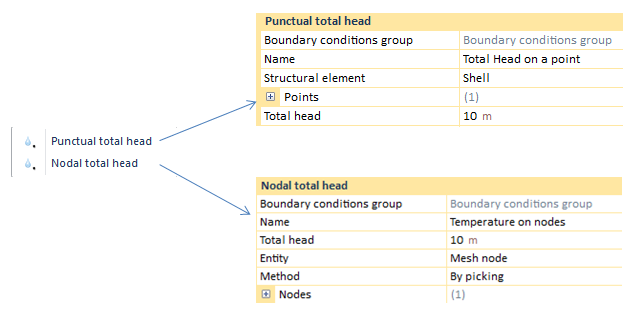
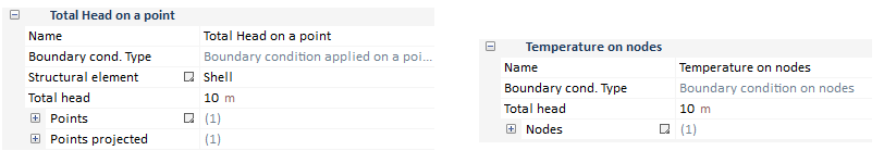
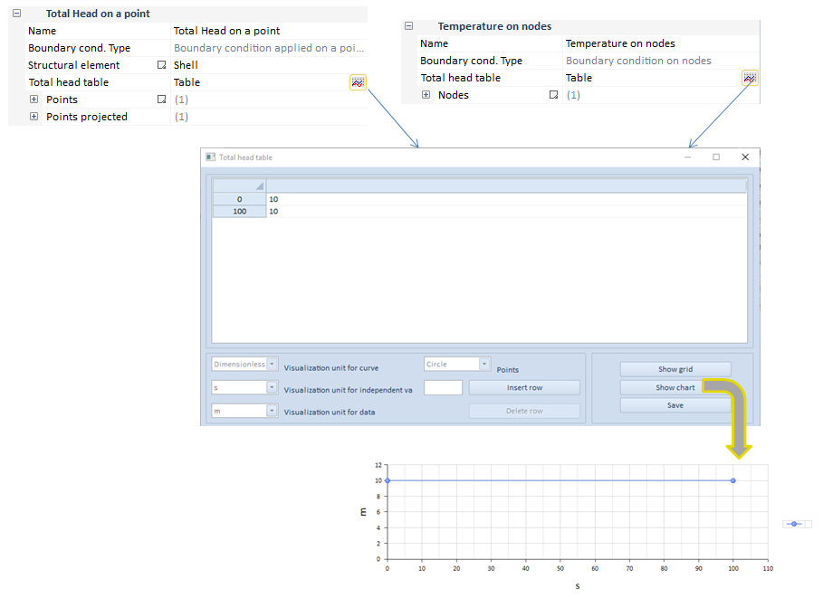
Punctual total head
Total head on curve
Total head on surface
Total head on volume
|
Length
|
|
Point flux
|
Length/time
|
|
Flux on surface
|
Length/time/Length^2
|
|
Flux on Volume
|
Length/time/Length^3
|
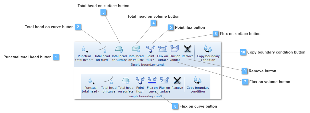
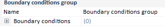
Total head on curve button
Add a total head on a curve to the group
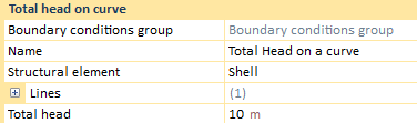
A boundary condition on a curve has loads per length unit and are applied over a curve attached to a line (truss or beam) or in the edges of a shell or a solid structural element. The calculated equivalent nodal forces are obtained by equally lumping the uniformly distributed loads onto the nodes.
This boundary condition would be valid both for 3D and 2D models.
Different linear loads applied at the same location are not accumulated, that is, CivilFEM solves the situation executing an average between the whole amount of seepage conditions, providing a single result.
Application of this type of boundary condition, depends on the analysis. For instance, if we have a static analysis the BC property bar does not change.
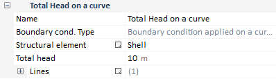
Required data for linear load application are:
On the other hand, in case of either transient analysis, some changes are applied.
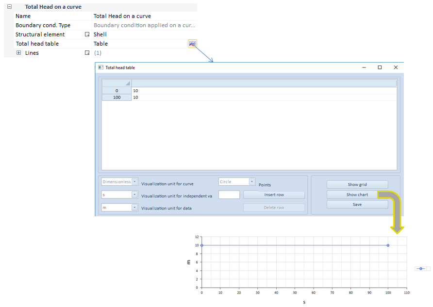
As it can be seen in this transient analysis example, the load is dependent on time.
| ||||||
Total head on surface button
Add a total head on a surface to the group
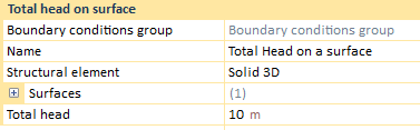
This option creates distributed seepage boundary condition/seepage loads over a surface attached to a shell or solid structural element. The calculated equivalent nodal forces are obtained by equally lumping the uniformly distributed loads onto the nodes.
Different seepage conditons on surface loads applied at the same location are not accumulated, that is, CivilFEM solves the situation executing an average between the whole amount of conditions, providing a single result.
This boundary condition would be valid both for 3D and 2D models.
Solid 3D
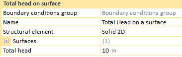
Solid 2D
If the current structural element is a shell, there will only be a surface in which the load can be applied. However, two different total head conditions may be entered, that is, a top total head and a bottom total head. This total head is applied on the surface nodes, being the target of entering two different total head the calculation of a seepage gradient on the width of the shell.
Shells
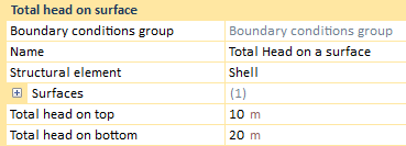
The previous described information about the shell data, takes part in the result process. When the solving process has finished and the results have been loaded, the user can see three different options in the "Result" drop: top total head, bottom total head and average total head.
The top and the bottom total heads will show the entered total head. Nevertheless, the average total head will come out an average value between both of the previous conditions. In addition, any time a shell structural element has been created, although any other structural element type exists, the "Result" drop will always provide a top, a bottom and an average total head.
On the other hand, if the created structural element is a solid, the user will only be able to choose a single surface to apply the total head on surface.
In this case, the "Result" drop will only output a total head result, as long as there is not a shell structural element in the entities of the model, the "Result" drop would only contain the global total head.
Application of this type of boundary condition, depends on the analysis. For instance, if we have a static analysis the BC property bar does not change.
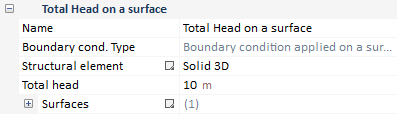
Required data for surface load application are:
On the other hand, in case of either transient analysis, some changes are applied.
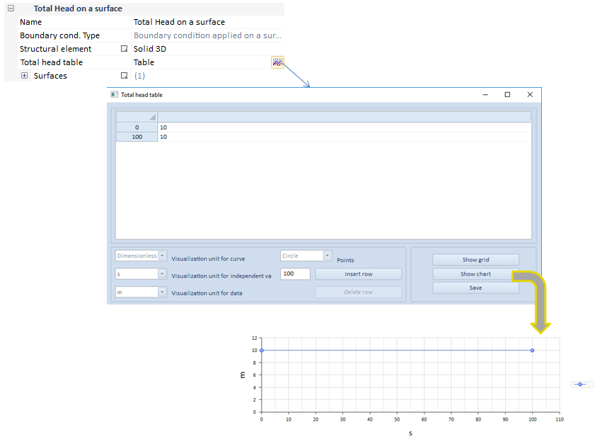
As it can be seen in this transient analysis example, the load is dependent on time.
| ||||||||
Total head on volume button
Add a total head on a volume to the group
This option creates distributed seepage boundary condition/total head loads over a volume attached to a solid structural element. The calculated equivalent nodal forces are obtained by equally lumping the uniformly distributed loads onto the nodes.
Different total heads on volume loads applied at the same location are not accumulated, that is, CivilFEM solves the situation executing an average between the whole amount of conditions, providing a single result.
This boundary condition is only available in 3D models.
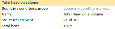
Application of this type of boundary condition, depends on the analysis. For instance, if we have a static analysis the BC property bar does not change.
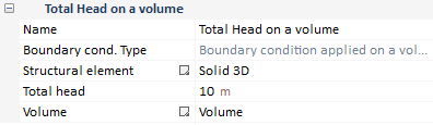
Required data for volumetric load application are:
On the other hand, in case of either transient analysis, some changes are applied.
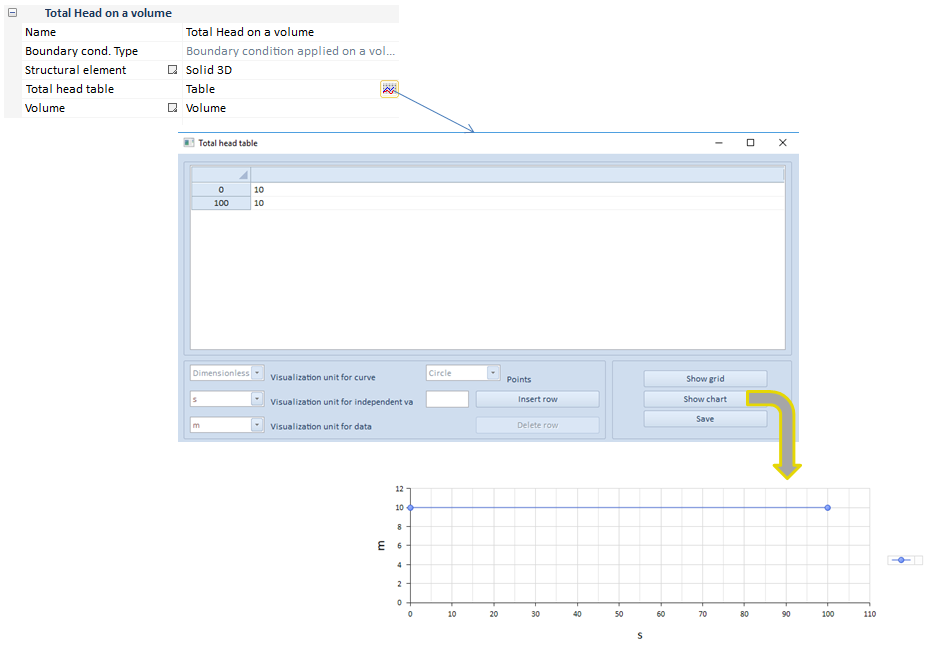
As it can be seen in this transient analysis example, the load is dependent on time.
| ||||||
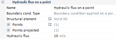
Point flux button
Add a point hydraulic flux to the group
The point flux utility creates a punctual flux on a list of points or nodes.
The point flux loads can also be defined at nodes, once the structural element has been meshed.
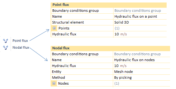
This boundary condition would be valid both for 3D and 2D models.
The main difference between creating a load by points is the use of geometry entities whereas, by nodes, the load is fixed on nodes of the structural element.
Most of the required data needed to create a punctual flux BC, both by points or nodes, will be defined below.
In regards to the point flux properties bar, it is subjected to change depending on the chosen analysis type.
For instance, if we have a static analysis, the flux properties bar does not change.
On the other hand, in the case of either a transient analysis, some changes are applied.
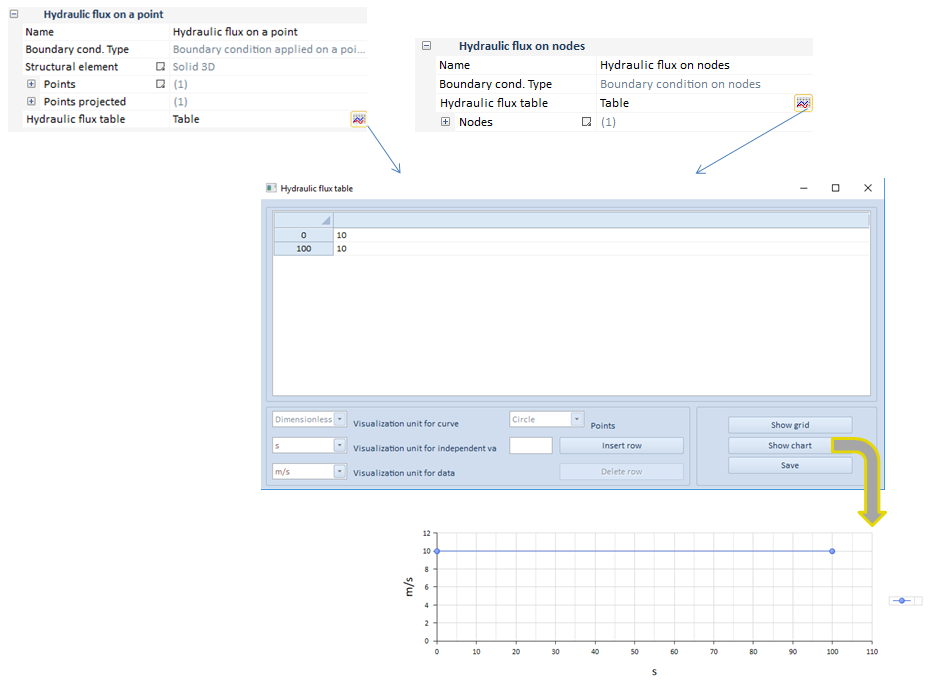
As it can be seen in this transient analysis example, the flux is dependent on time.
When the user sets two or more different fluxes on the same point, CivilFEM solves the situation executing the addition of the whole amount of fluxes, providing a single result.
On another note, last but not least important is the concept of seepage face review, as well. This tool is only available when applying a nodal flux. It consist of a check box that will be capable of being active or deactivated in the nodal flux properties bar.
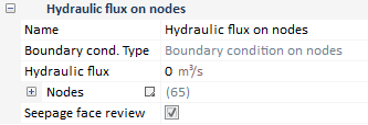
One of the problems with the seepage faces is its size due to the possibility of being not known so, it would become necessary to determine it by means of a process of iteration.
The seepage face review tool allows selecting a list of nodes on which the seepage face may be carried out, in relation with the other boundary conditions which perform the case study. The definition of a hydraulic flux is really important due to the fact that this implies over which value the solver is going to iterate so as to find the seepage face. This value is usually 0 because it correspond to the water table value, or a pore pressure value of 0. However, this initially-specified flux may be some other positive or negative value. a positive value could represent infiltration and a negative value could represent evaporation.
The algorithm behavior is developed taking into account the provided hydraulic flux. In case this value is 0, this means we are looking for the water table. For this purpose, the program evaluates the condition of H=y all over the seepage face nodes, being H their total head value and y their height. As a result of this, the condition of a positive pressure on any of the seepage face nodes could not happen, due to the fact that the water flux should not be able to pond into the soil.
Therefore the solver will iterate as many times as necessary discarding all those nodes on which the flux is positive and the condition of H=y are not fulfilled. This process will be completed when the program finds all the nodes with these conditions, as long as the iterations does not exceed the max. iteration number specified in the solution controls.
This action will be performed by Load Case, as long as a boundary condition of seepage face review has been added to them. In a transient analysis, the size of the review seepage face must be determined separately for each time step.
A new case study of seepage in a dam is performed. The problem consists of a dam with some boundary conditions, that is, the red line corresponds to a total head of 10 m, the yellow point is a total head of 0 and the green line is the so called seepage face review boundary condition. The results visualization will be carried out ahead:
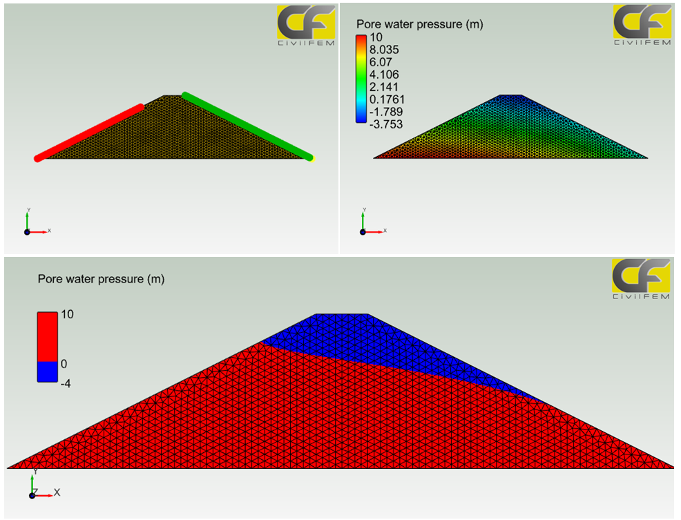
The last image pretends an easygoing visualization of the water table, being this one the line which separate the blue and the red area, which corresponds to the line with a pore water pressure of 0.
| ||||||||||
Flux on surface button
Add a hydraulic flux on a volume to the group
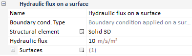
The flux on surface utility creates a flux all over a surface, that is, the hydraulic vector flux is defined for this surface. This type of flux may be applied on faces of a solid or the face of a shell.
When the user sets two or more different fluxes on the same surface, CivilFEM solves the situation executing the addition of the whole amount of fluxes, providing a single result.
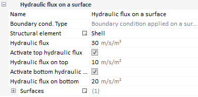
The application vary depending on if the structural element is a solid or a shell. When a solid is modeled, only a hydraulic flux is able to be entered, while in a shell, three different fluxes might be inputted.
This boundary condition would be valid both for 3D and 2D models.
Solid 3D
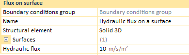
The hydraulic flux to apply correspond to a superficial one, entered on one, or more, solid surfaces.
Solid 2D
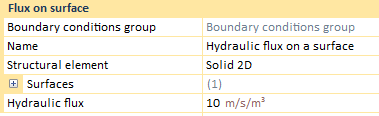
The hydraulic flux on a surface, for a 2D model, would be defined as a velocity per volume instead of a velocity per surface.
Shells
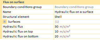
When the modeled structural element is a shell, three different fluxes can be defined. Top and bottom fluxes correspond to superficial fluxes due to be structured as a 3D element, while the "Hydraulic flux" is based on an volumetric heat density.
Most of the required data needed to create a punctual flux BC, both by points or nodes, will be defined below.
In regards to the flux on surface properties bar, it is subjected to change depending on the chosen analysis type.
For instance, if we have a static analysis, the flux properties bar does not change.
Solid
Shells
On the other hand, in the case of either a transient analysis, some changes are applied.
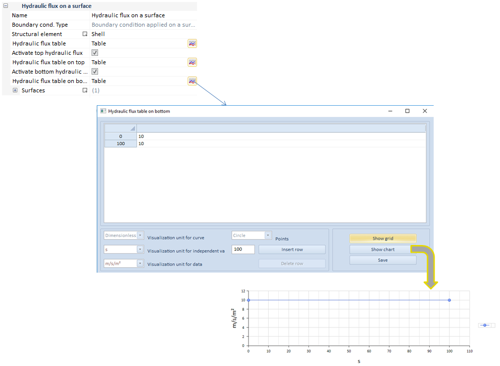
As it can be seen in this transient analysis example, the flux is dependent on time. In case of being a shell structural element, the three values would be dependent of time, both the top and the bottom values, and the volumetric heat density.
| ||||||
Flux on volume button
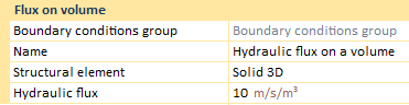
Add a hydraulic flux on a volume to the group
The flux on volume utility creates a flux all over a volume, that is, the hydraulic vector flux is defined for this volume. This type of flux is only available for a solid structural element, therefore it is an option only allowed in a 3D model.
When the user sets two or more different fluxes on the same volume, CivilFEM solves the situation executing the addition of the whole amount of fluxes, providing a single result.
Application of this type of boundary condition, depends on the analysis. For instance, if we have a static analysis the BC property bar does not change.
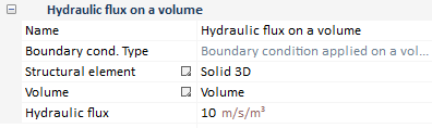
Required data for volumetric heat density application are:
On the other hand, in case of either transient analysis, some changes are applied.
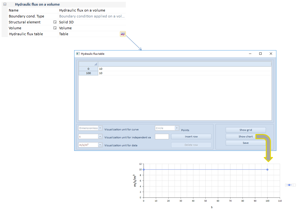
As it can be seen in this transient analysis example, the volumetric heat density is dependent on time.
| ||||||
Flux on curve button
Add a hydraulic flux on a curve to the group
The flux on volume utility creates a flux all over a volume, that is, the thermal vector flux is defined for this volume. This type of flux is only available for a solid structural element, therefore it is an option only allowed in a 3D model.
When the user sets two or more different fluxes on the same curve, CivilFEM solves the situation executing the addition of the whole amount of fluxes, providing a single result.
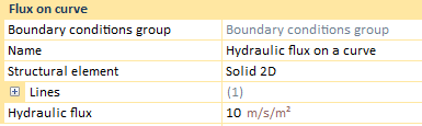
Application of this type of boundary condition, depends on the analysis. For instance, if we have a static analysis the BC property bar does not change.
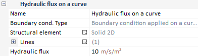
Required data for volumetric heat density application are:
On the other hand, in case of either transient analysis, some changes are applied.
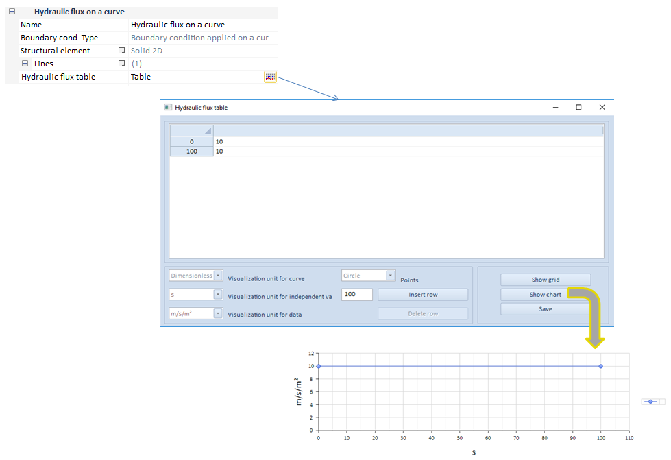
As it can be seen in this transient analysis example, the flux is dependent on time.
| ||||||