|
|||||
|
|||||||
|
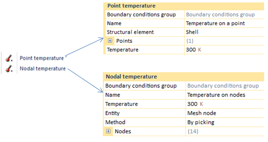
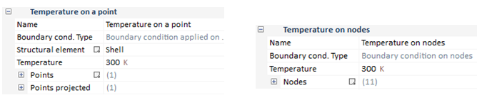
Point temperature
Temperature on curve
Temperature on surface
Temperature on volume
|
Temperature
|
|
Point flux
|
Power
|
|
Flux on surface
|
Power/Length^2
|
|
Flux on Volume
|
Power/Length^3
|
|
Film coefficient on surface (h coefficient)
|
Power/(Length^2 · temperature)
|
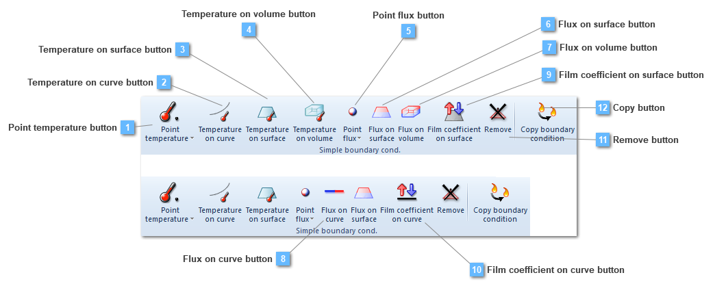
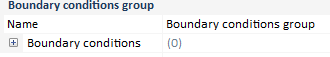
Temperature on curve button
Add a temperature on a curve to the group
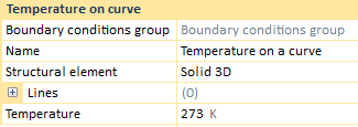
A boundary condition on a curve has loads per length unit and are applied over a curve attached to a linear (truss or beam) or in the edges of a shell or a solid structural element. The calculated equivalent nodal forces are obtained by equally lumping the uniformly distributed loads onto the nodes.
This boundary condition would be valid both for 3D and 2D models.
Different linear loads applied at the same location are not accumulated, that is, CivilFEM solves the situation executing an average between the whole amount of temperatures, providing a single result.
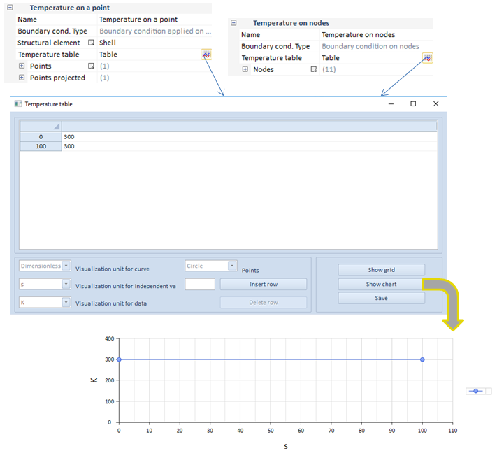
Application of this type of boundary condition, depends on the analysis. For instance, if we have a static analysis the BC property bar does not change.
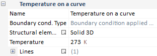
Required data for linear load application are:
On the other hand, in case of either transient analysis, some changes are applied.
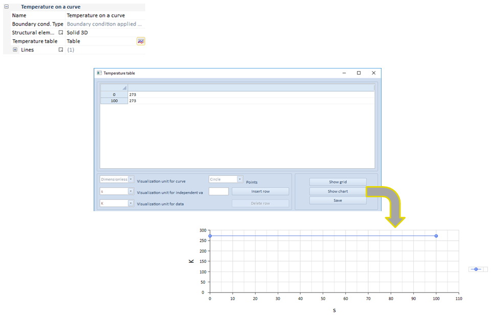
As it can be seen in this transient analysis example, the load is dependent on time.
| ||||||
Temperature on surface button
Add a temperature on a surface to the group
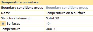
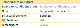
This option creates distributed thermal boundary condition/thermal loads over a surface attached to a shell or solid structural element. The calculated equivalent nodal forces are obtained by equally lumping the uniformly distributed loads onto the nodes.
Different temperature on surface loads applied at the same location are not accumulated, that is, CivilFEM solves the situation executing an average between the whole amount of temperatures, providing a single result.
This boundary condition would be valid both for 3D and 2D models.
Solid 3D
Solid 2D
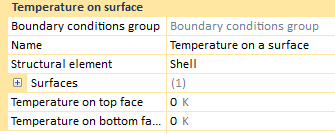
If the current structural element is a shell, there will only be a surface in which the load can be applied. However, two different temperatures may be entered, that is, a top temperature and a bottom temperature. This temperature is applied on the surface nodes, being the target of entering two different temperatures the calculation of a thermal gradient on the width of the shell.
Shells
The previous described information about the shell data, takes part in the result process. When the solving process has finished and the results have been loaded, the user can see that in the "Result" drop, three different options are visualized:
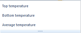
The top and the bottom temperature will show the entered temperatures. Nevertheless, the average temperature will come out an average value between both of the previous temperatures. In addition, any time a shell structural element has been created, although any other structural element type exists, the "Result" drop will always provide a top, a bottom and an average temperature.
On the other hand, if the created structural element is a solid, the user will only be able to choose a single surface to apply the temperature on surface.
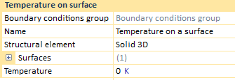
In this case, the "Result" drop will only output a temperature result, as long as there is not a shell structural element in the entities of the model.
Application of this type of boundary condition, depends on the analysis. For instance, if we have a static analysis the BC property bar does not change.
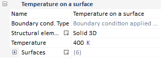
Required data for surface load application are:
On the other hand, in case of either transient analysis, some changes are applied.
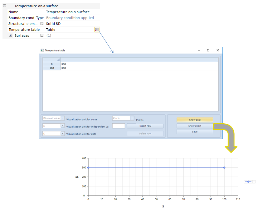
As it can be seen in this transient analysis example, the load is dependent on time.
| ||||||||
Temperature on volume button
Add a temperature on a volume to the group
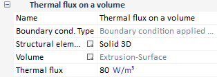
This option creates distributed thermal boundary condition/thermal loads over a volume attached to a solid structural element. The calculated equivalent nodal forces are obtained by equally lumping the uniformly distributed loads onto the nodes.
Different temperature on volume loads applied at the same location are not accumulated, that is, CivilFEM solves the situation executing an average between the whole amount of temperatures, providing a single result.
This boundary condition is only available in 3D models.
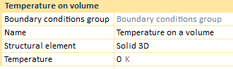
Application of this type of boundary condition, depends on the analysis. For instance, if we have a static analysis the BC property bar does not change.
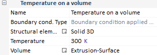
Required data for volumetric load application are:
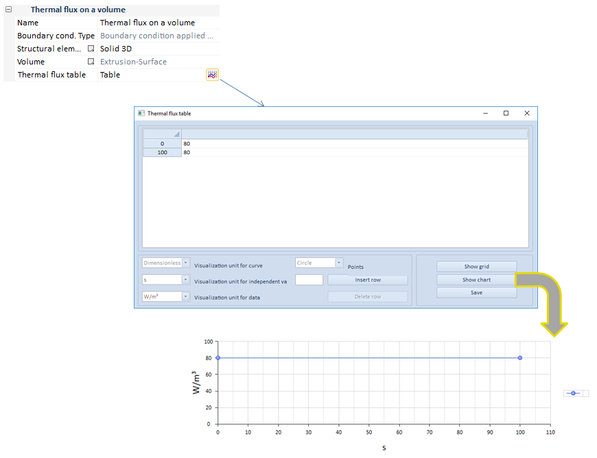
On the other hand, in case of either transient analysis, some changes are applied.
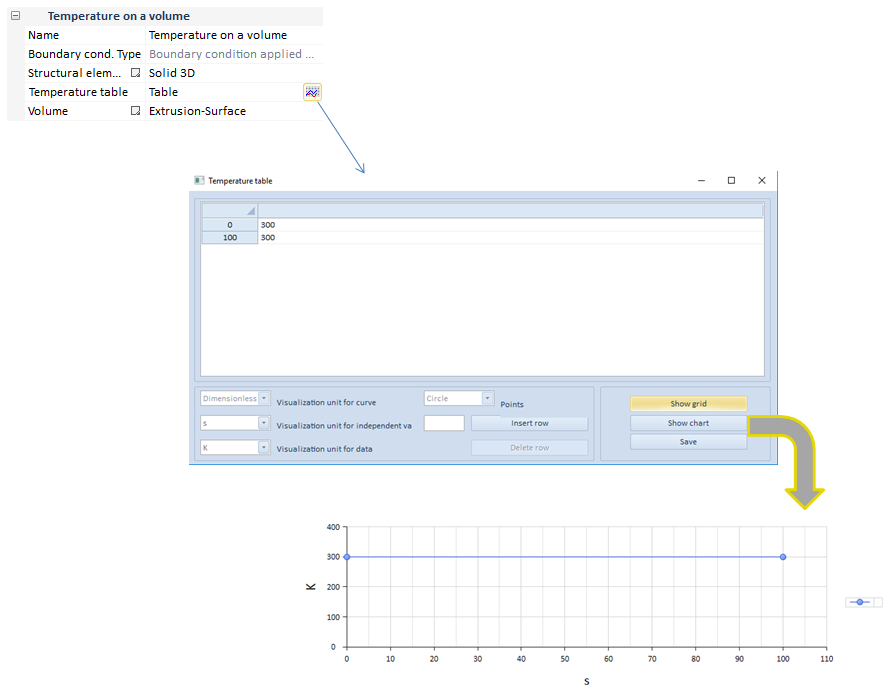
As it can be seen in this transient analysis example, the load is dependent on time.
| ||||||
Point flux button
Add a point flux to the group
The point flux utility creates a punctual flux on a list of points or nodes.
The point flux loads can also be defined at nodes, once the structural element has been meshed.
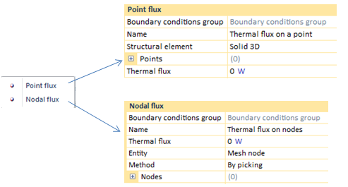
This boundary condition would be valid both for 3D and 2D models.
The main difference between creating a load by points is the use of geometry entities whereas, by nodes, the load is fixed on nodes of the structural element.
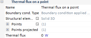
Most of the required data needed to create a punctual flux BC, both by points or nodes, will be defined below.
In regards to the point flux properties bar, it is subjected to change depending on the chosen analysis type.
For instance, if we have a static analysis, the flux properties bar does not change.
On the other hand, in the case of either a transient analysis, some changes are applied.
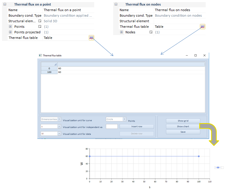
As it can be seen in this transient analysis example, the flux is dependent on time.
When the user sets two or more different fluxes on the same point, CivilFEM solves the situation executing the addition of the whole amount of fluxes, providing a single result.
| ||||||||
Flux on surface button
Add a flux on a surface to the group
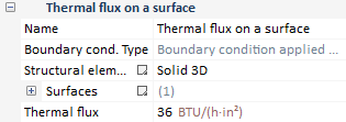
The flux on surface utility creates a flux all over a surface, that is, the thermal vector flux is defined for this surface. This type of flux may be applied on faces of a solid or the face of a shell.
When the user sets two or more different fluxes on the same surface, CivilFEM solves the situation executing the addition of the whole amount of fluxes, providing a single result.
The application vary depending on if the structural element is a solid or a shell. When a solid is modeled, only a thermal flux is able to be entered, while in a shell, three different fluxes might be inputted.
This boundary condition would be valid both for 3D and 2D models.
Solid 3D
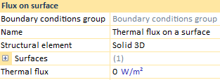
The thermal flux to apply correspond to a superficial one, entered on one, or more, solid surfaces.
Solid 2D
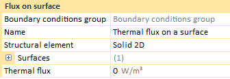
The thermal flux on a surface, for a 2D model, would be defined as a volumetric heat density instead of a superficial one.
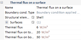
Shells
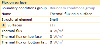
When the modeled structural element is a shell, three different fluxes can be defined. Top and bottom fluxes correspond to superficial fluxes due to be structured as a 3D element, while the "Thermal flux" is based on an volumetric heat density.
Most of the required data needed to create a punctual flux BC, both by points or nodes, will be defined below.
In regards to the flux on surface properties bar, it is subjected to change depending on the chosen analysis type.
For instance, if we have a static analysis, the flux properties bar does not change.
Solid
Shells
On the other hand, in the case of either a transient analysis, some changes are applied.
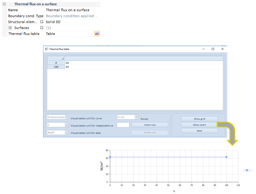
As it can be seen in this transient analysis example, the flux is dependent on time. In case of being a shell structural element, the three values would be dependent of time, both the top and the bottom values, and the volumetric heat density.
| ||||||
Flux on volume button
Add a flux on a volume to the group
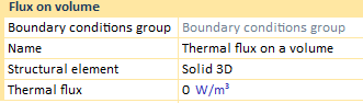
The flux on volume utility creates a flux all over a volume, that is, the thermal vector flux is defined for this volume. This type of flux is only available for a solid structural element, therefore it is an option only allowed in a 3D model.
When the user sets two or more different fluxes on the same volume, CivilFEM solves the situation executing the addition of the whole amount of fluxes, providing a single result.
Application of this type of boundary condition, depends on the analysis. For instance, if we have a static analysis the BC property bar does not change.
Required data for volumetric heat density application are:
On the other hand, in case of either transient analysis, some changes are applied.
As it can be seen in this transient analysis example, the volumetric heat density is dependent on time.
| ||||||
Flux on curve button
Add a flux on a curve to the group
The flux on volume utility creates a flux all over a volume, that is, the thermal vector flux is defined for this volume. This type of flux is only available for a solid structural element, therefore it is an option only allowed in a 3D model.
When the user sets two or more different fluxes on the same curve, CivilFEM solves the situation executing the addition of the whole amount of fluxes, providing a single result.
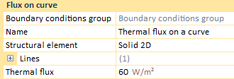
Application of this type of boundary condition, depends on the analysis. For instance, if we have a static analysis the BC property bar does not change.
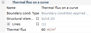
Required data for volumetric heat density application are:
On the other hand, in case of either transient analysis, some changes are applied.
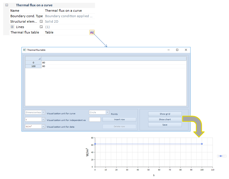
As it can be seen in this transient analysis example, the flux is dependent on time.
| ||||||
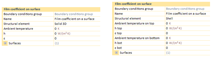
Film coefficient on surface button
Add a film coefficient on a surface to the group
The film coefficient is the a constant which may be calculated by the quotient of the heat flux and the thermodynamic driving force for the flow heat.

There are some differences between models 3D and 2D when the film coefficient is applied. That is, if the user applies the film coefficient on a surface, the model can only be a 3D model, whereas if the model correspond to a 2D one, the user will only be able to apply this coefficient on curves.
In addition, on a 3D model, the situation is much different if the structural element correspond to a solid or if, by contrary, it is a shell. When a solid is modeled, the h coefficient is exclusive but in shells, h coefficient is distinguished through h top and h bottom.
Application of this type of boundary condition, depends on the analysis. For instance, if we have a static analysis the BC property bar does not change.
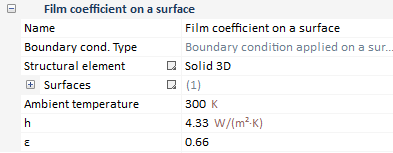
Required data for the film coefficient application are:
On the other hand, in case of either transient analysis, some changes are applied.
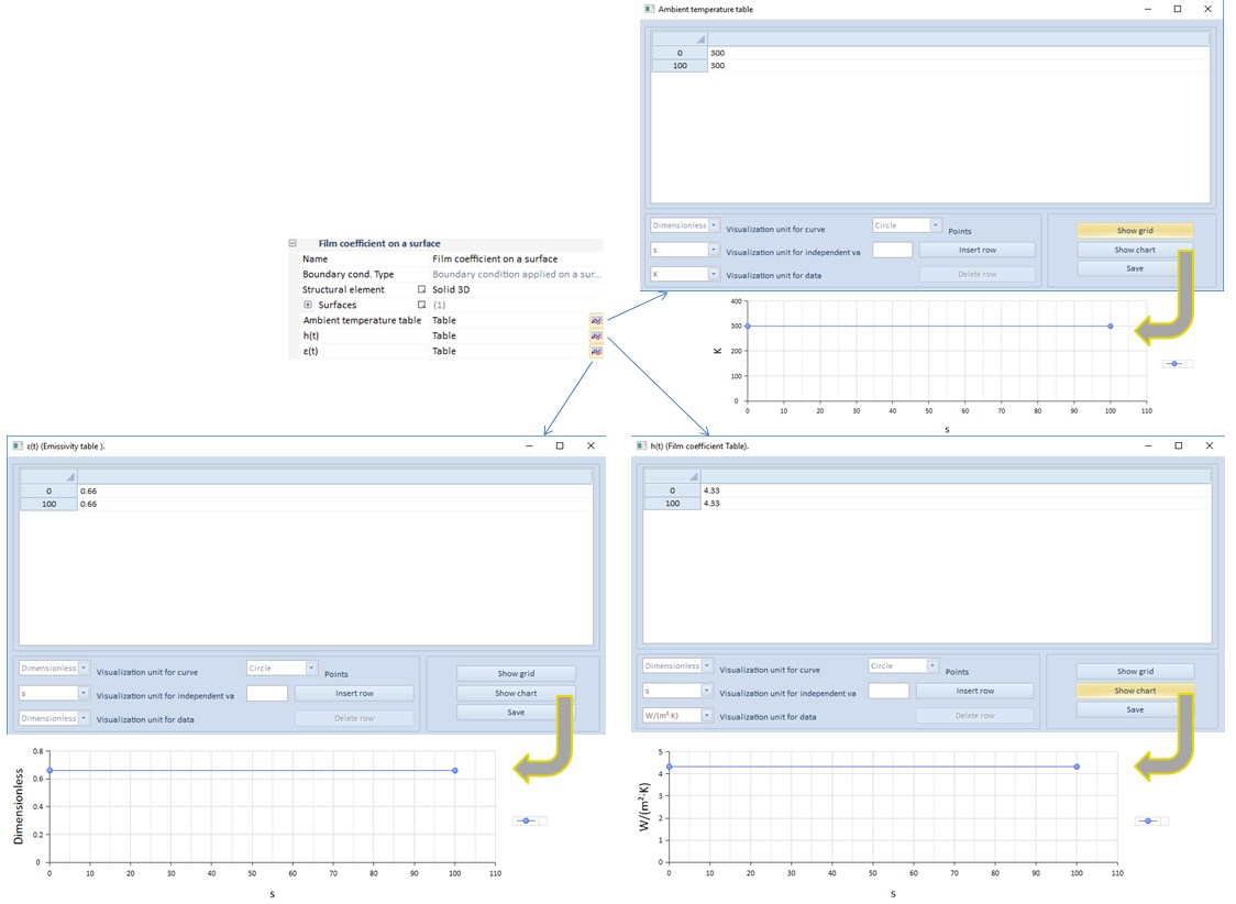
As it can be seen in this transient analysis example, both the film coefficient and the ambient temperature are dependent on time.
On a separate issue, it could be interesting to analyze how the film condition is taken so, ahead, a little scheme has been plotted but also the main equation can be seen as well.
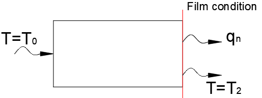
On that face or curve, a film condition has been imposed, therefore, a flux qn is taking place.
This equation is shaped by some parameters:
It will be the user who must enter the T0 temperature, while the T2 will be the required condition to solve the problem.
| ||||||||||
Film coefficient on curve button
Add a film coefficient on a curve to the group
The film coefficient is the a constant which may be calculated by the quotient of the heat flux and the thermodynamic driving force for the flow heat.
There are some differences between models 3D and 2D when the film coefficient is applied. That is, if the user applies the film coefficient on a surface, the model can only be a 3D model, whereas if the model correspond to a 2D one, the user will only be able to apply this coefficient on curves.
This boundary condition would be applied on any curve, whether one-dimensional structural elements or over lines of a two-dimensional structural elements.
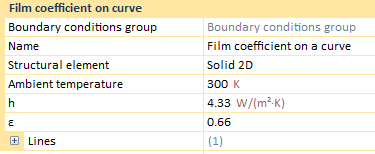
For instance, a Solid 2D properties bar would be visualized:
Application of this type of boundary condition, depends on the analysis. For instance, if we have a static analysis the BC property bar does not change.
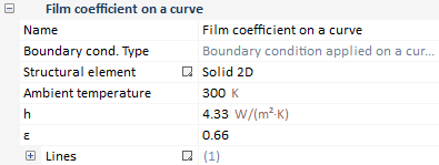
Required data for the film coefficient application are:
On the other hand, in case of either transient or harmonic analysis, some changes are applied.
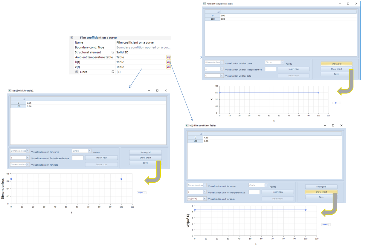
As it can be seen in this transient analysis example, both the film coefficient and the ambient temperature are dependent on time.
On a separate issue, it could be interesting to analyze how the film condition is taken so, ahead, a little scheme has been plotted but also the main equation can be seen as well.
On that face or curve, a film condition has been imposed, therefore, a flux qn is taking place.
This equation is shaped by some parameters:
It will be the user who must enter the T0 temperature, while the T2 will be the required condition to solve the problem.
| ||||||||||