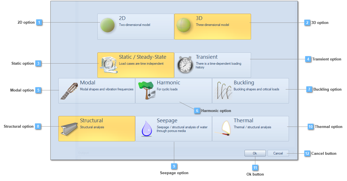
Menu

Dialog

Dialog
1

2D option

1. 2D option
 
Option with which a new 2D model is created.
 
2

3D option

2. 3D option
 
Create a new 3D model.
 
3

Static option

3. Static option
 
The static analysis option provides the most basic analysis of a structural model. All the applied loads will be "static", meaning that they will stay constant during all the calculation time. The static option is used for analyzing structural models under non-moving loads. It can be also used to perform a check/design by code.
 
A static analysis can include non-linearities, but they can't be time dependent.
 
After static analysis has been done, other analysis can be performed on the same model, such as a dynamic analysis for studying a time dependent response of the structure. In computer terminology, static means fixed, while dynamic means capable of action and/or change.
 
This static FEA is regularly used to verify whether the current design meets infinite life time under working conditions or not by combining the stress calculation result with theory of failure that includes safety factor.
 
4

Transient option

4. Transient option
 
Transient dynamic analysis deals with an initial-boundary value problem. In order to solve the equations of motion of a structural system, it is important to specify the proper initial conditions and boundary conditions. You obtain the solution to the equations of motion by using either modal superposition (for linear systems) or direct integration (for linear or nonlinear systems). In direct integration, selecting a proper time step is very important. For both methods, you can include damping in the system.
 
The basic equation of motion solved by a transient dynamic analysis is:
 
 
Where:
 
[M] = mass matrix
[C] = damping matrix
[K] = stiffness matrix
= nodal acceleration vector
= nodal velocity vector
= nodal displacement vector
{F(t)} = load vector
 
At any given time, t, these equations can be thought of as a set of "static" equilibrium equations that also take into account inertia forces ([M]) and damping forces ([C]). CivilFEM grants the option of choosing between either the Newmark or the α generalized time integration methods to solve these equations at discrete timepoints. The time increment between successive timepoints is called the integration time step.
 
Three methods are available to do a transient dynamic analysis:
 
  • The Full Method
  • The Reduced Method
  • The Mode Superposition Method
 
The Full Method will be explained below.
 
The Full Method uses the full system matrices to calculate the transient response (no matrix reduction). It is the most powerful of the three methods because it allows all types of nonlinearities to be included (plasticity, large deflections, large strain, etc.).
 
The advantages of the full method are:
 
  • It is easy to use, because you don't have to worry about choosing master degrees of freedom or mode shapes.
  • It allows all types of nonlinearities.
  • It uses full matrices, so no mass matrix approximation is involved.
  • All displacements and stresses are calculated in a single pass.
  • It accepts all types of loads: nodal forces, imposed (non-zero) displacements (although not recommended), and element loads (pressures and temperatures).
  • It allows effective use of solid-model loads.
     
5

Modal option

5. Modal option
 
CivilFEM uses the Lanczos method to extract eigenvalues (natural frequencies) and eigenvectors (mode shapes), optimal for several modes. After the modes are extracted, they can be used in a transient analysis or spectrum response calculation.
 
In dynamic eigenvalue analysis, we find the solution to an undamped linear dynamics problem:
 
Where K is the stiffness matrix, M is the mass matrix, are the eigenvalues (frecuencies) and are the eigenvectors. In CivilFEM, if the extraction is performed after increment zero, K is the tangent stiffness matrix, which can include material and geometrically nonlinear contributions. The mass matrix is formed from both distributed mass and point masses.
 
The Lanczos algorithm converts the original eigenvalue problem into the determination of the eigenvalues of a tri-diagonal matrix. The method can be used either for the determination of all modes or for the calculation of a small number of modes. For the latter case, the Lanczos method is the most efficient eigenvalue extraction algorithm. A simple description of the algorithm is as follows. Consider the eigenvalue problem:
 
Previous equation can be rewritten as:
 
 
Inside CivilFEM either the number of modes or a range of modes to be extracted can be selected. The Sturm sequence check can be used to verify that all of the required eigenvalues have been found.
 
In addition, the user can select the lowest frequency to be extracted, greater than zero.
 
Eigenvalue extraction is controlled by the maximum number of iterations for all modes in the Lanczos iteration method.
 
6

Harmonic option

6. Harmonic option
 
Any sustained cyclic load will produce a sustained cyclic response in a structural system. Harmonic response analysis gives the ability to predict the sustained dynamic behavior of structures, thus enabling to verify whether or not designs will successfully overcome resonance, fatigue, and other harmful effects of forced vibrations.
 
Harmonic response analysis allows the analysis of structures vibrating around an equilibrium state. This equilibrium state can be free or statically prestressed. Statically prestressed equilibrium states can include material and/or geometric nonlinearities. The user can compute the damped response for prestressed structures at various states.
 
In many practical applications, components are dynamically excited. These dynamic excitations are often harmonic and usually cause only small amplitude vibrations. CivilFEM linearizes the problem around the equilibrium state. If the equilibrium state is a nonlinear, statically prestressed situation, CivilFEM considers all effects of the nonlinear deformation on the dynamic solution. These effects include the following:
 
  • Initial stress.
  • Change of geometry.
  • Influence on constitutive law.
     
The vibration problem can be solved as a linear problem using complex arithmetic.
 
The analytical procedure consists of the following steps:
 
-CivilFEM calculates the response of the structure to a static preload (which can be nonlinear) based on the constitutive equation for the material response. In this portion of the analysis, the program ignores inertial effects.
 
-CivilFEM calculates the complex-valued amplitudes of the superimposed response for each given frequency, and amplitude of the boundary tractions and/or displacements. In this portion of the analysis, the program considers both material behavior and inertial effects.
 
-It is also possible to apply different loads with different frequencies or change the static preload at your discretion. All data relevant to the static response is stored during calculation of the complex response.
 
A harmonic analysis, by definition, assumes that any applied load varies harmonically (sinusoidally) with time. To completely specify a harmonic load, three pieces of information are usually required: the amplitude, the phase angle, and the forcing frequency range.
 
The amplitude is the maximum value of the load.
 
The phase angle is a measure of the time by which the load lags (or leads) a frame of reference. On the complex, it is the angle measured from the real axis. The phase angle is required only if you have multiple loads that are out of phase with each other.
                                  
7

Buckling option

7. Buckling option
 
Evaluation of structural buckling must be taken into account due to the importance of this effect in slender structures that could cause the a structural failure. Buckling happens suddenly, without little if any prior warning, so there is almost no chance for corrective action.
 
Buckling of a structure happens when the stiffness matrix approaches a singular value. You can extract the eigenvalue in a linear analyses to obtain the linear buckling load. You can also perform eigenvalue analysis for a buckling load in a nonlinear problem based on the incremental stiffness matrices.
 
Inside the internal structure of a buckling analysis, it is also possible to perform either a linear buckling analysis or a non-linear buckling analysis, depending on the structural composition.
 
Linear buckling analysis.
 
First, consider a linear-buckling analysis (also called eigenvalue-based buckling analysis), that is in many ways similar to a modal analysis. Linear buckling is the most common type of analysis and is easy to execute, but it is limited in the results it can provide.
 
Linear buckling analysis calculates the buckling load magnitudes that cause buckling and associated buckling modes.
 
FEA (finite element analysis) programs provide calculations of a large number of buckling modes and the associated buckling-load factors (BLF). The BLF is expressed by a number that factored by the applied load gives the total buckling-load magnitude.
 
The buckling mode presents the shape the structure assumes when it buckles in a particular mode, but says nothing about the numerical values of the displacements or stresses. The numerical values can be displayed, but are merely relative. This is in close analogy to modal analysis, that calculates the natural frequency and provides qualitative information on the modes of vibration (modal shapes), but not on the actual magnitude of displacements.
 
Theoretically, it is possible to calculate as many buckling modes as the number of degrees of freedom in the FEA model. Most often, though, only the first positive buckling mode and its associated BLF need be found. This is because higher buckling modes have no chance of taking place — buckling most often causes catastrophic failure or renders the structure unusable.
 
Nonlinear buckling analysis.
 
As with any other nonlinear analysis, nonlinear-buckling analysis requires that a load is applied gradually in multiple steps rather than in one step as in a linear analysis. Each load increment changes the structure shape, and this, in turn, changes the structure stiffness. Therefore, the structure stiffness must be updated at each increment.
 
When buckling happens, the structure undergoes a momentary loss of stiffness and the load control method would result in numerical instabilities. Nonlinear buckling analysis requires another way of controlling load application. Here, points corresponding to consecutive load increments are evenly spaced along the load-displacement curve, which itself is constructed during load application.
 
In contrast to linear-buckling analysis, that only calculates the potential buckling shape with no quantitative values of importance, nonlinear analysis calculates actual displacements and stresses.
 
The buckling option solves the following eigenvalue problem by either the inverse power sweep or the Lanczos method:
 
 
Where is assumed to be a linear function of the load increment to cause buckling.
 
The geometric stiffness used for the buckling load calculation is based on the stress and displacement state change at the start of the last increment. However, the stress and strain states are not updated during the buckling analysis.
 
8

Structural option

8. Structural option
 
Structural analysis is the process determined by a structural effect in relation with a load system. This structural response is, generally, taken into account for sizing both the inner forces and the structural deformations.
 
It is also possible to say that the structural calculation model is defined by:
 
  • Geometry
  • Boundary conditions
  • Materials
  • Loads
 
The structural analysis option is chosen as long as seepage and thermal analysis are not required.
 
9

Seepage option

9. Seepage option
 
The seepage capability allows the user to obtain total head distributions, in a structure, for linear and nonlinear problems in relation to seepage conditions. This is also possible for one, two and three dimensional elements both in a steady-state and in a transient analysis.
 
Elements which take part in this analysis process, are compatible with elements of stress, that is the reason why the same mesh can be used for both the seepage and the structural model.
 
The nonlinearities may include saturated/unsaturated hydraulic properties and thermal contacts.
 
The hydraulic conductivity can be either isotropic or orthotropic, being managed to be defined a different hydraulic conductivity for each direction.
 
A Seepage analysis is carried out as long as it becomes necessary to evaluate the total head, or even any seepage condition, all over a soil but also a specific structure.
 
10

Thermal option

10. Thermal option
 
The heat transfer capability allows the user to obtain temperature distributions, in a structure, for linear and nonlinear heat transfer problems. This is also possible for one, two and three dimensional elements both in a steady-state and in a transient analysis.
 
Elements which take part in this analysis process, are compatible with elements of stress, that is the reason why the same mesh can be used for both the heat transfer and the structural model.
 
The nonlinearities may include temperature-dependent properties, latent heat effect, heat convection in the flow direction, thermal contacts and nonlinear boundary conditions such as convection and radiation.
 
In addition, in case the temperature-dependent check box is active, it will be also possible to establish a temperature dependency function.
 
The thermal conductivity can be either isotropic or orthotropic, being managed to be defined a different thermal conductivity for each direction.
 
A Thermal analysis is carried out as long as it becomes necessary to evaluate how the heat transfer behaves in a structure.
 
11

Ok button

11. Ok button
 
Order the execution
 
12

Cancel button

12. Cancel button
 
Cancel execution