14.1                 Introduction

Seismic design with CivilFEM provides the user a set of tools to analyze seismic action on structures, according to the provisions of:

• Eurocode 8
• The Spanish codes NCSE-94 and NCSE-02
• The Chinese code GB50011
• The Italian code ITA3274
• AASHTO LRFD Bridge Design Specifications
• The Greek code EAK 2000
• CALTRANS Seismic Design Criteria
• Uniform Building Code (1997)
• The French code PS 92
• Indian Standard 1893

 

Aspects considered for calculations:

1.    Spectrum definition

2.    Calculation of mode shapes

3.    Modal combination

Aspects 2 and 3 can be calculated with CivilFEM or with ANSYS directly for increased control over the methods used for obtaining the mode shapes or the mode combinations.

If the mode combination is performed directly with ANSYS, the ‘data set’ corresponding to the combined modes will not be written in CivilFEM’s results file. Therefore, in order to be able to perform operations in CivilFEM’s postprocessor at a later time, this ‘data set’ should be written in CivilFEM’s results file using the ~CFRAPPN command.

14.2                 Spectrum Calculation according to Eurocode 8 (ENV-1998-1-1:1994)

CivilFEM builds and defines the response spectrum in ANSYS from parameters through the following steps.

14.2.1                  Input data

The data required to define the response spectrum are input into the CivilFEM database with the ~DEFSPEC command.

The required data are listed below:

 

14.2.2                  Calculation of the Parameters for the Spectrum Definition

Once the data have been input, the fraction a is obtained by dividing the design ground acceleration a_g by the gravity acceleration g, displayed below:

14.2.3                  Spectrum Calculation

The values of the parameters which describe the response spectrum are given in the table below, in accordance with the subsoil type:

 

Table 14.2‑1 Values which describe the response spectrum

A total of 20 points of the spectrum are defined as shown below:

1.    Assignment of 7 fixed values of period T at the points where slope changes:

2.   The values of the 7 periods obtained up until this step are organized in ascending order.

3.   The ordinates of the vertical spectrum corresponding to each value of the period are calculated:

If the spectrum is linear, the ordinates of the horizontal spectrum are obtained as follows:

                                                                 

                                                                 

                                                                 

 

where:

q	=	behavior factor. The values of this factor are different for the horizontal seismic action and the vertical seismic action. Therefore, this factor assumes two different values qh and qv depending on the material type.
Kd1, Kd2	=	exponents which influence the shape of the design spectrum for a vibration period greater than TC, TD respectively.

For the elastic spectrum, the ordinates of the horizontal spectrum are obtained as follows:

                                                                 

where:

h	=	damping correction factor with reference value of h = 1 for a viscous damping of 5%.
K1, K2	=	exponents which influence the shape of the design spectrum for a vibration period greater than TC, TD respectively.

4.   For vertical movements, the response spectrum is the same as for horizontal seismic action, however, the ordinates are reduced as follows:

For vibrating periods T smaller than 0.15 s, a factor of 0.70 is used.

For vibrating periods T greater than 0.50 s, a factor of 0.50 is used.

For vibrating periods T between 0.15 s and 0.50 s, a linear interpolation shall be performed.

5.   Once the ordinates of the vertical spectrum have been calculated for the 7 points of the previous steps, the remaining 13 values of the period are calculated; thus the final total of 20 points will be achieved. The procedure for obtaining these 13 values is based on concentrating a greater number of values in sections with the highest absolute value of the slope.

6.   Once the 20 values of the period are determined, the corresponding values of the ordinates of the spectrum are calculated for both the horizontal and vertical components.

 

 

14.3                 Spectrum Calculation according to Eurocode 8 (EN-1998-1:2004)

CivilFEM builds and defines the response spectrum in ANSYS from required parameters through the following steps.

14.3.1                  Input Data

Data required to define the response spectrum are input into the CivilFEM database with the ~DEFSPEC command.

The required data are listed below:

 

14.3.2                  Calculation of the Parameters for the Spectrum Definition

 

Once the data have been input, the fraction a is obtained by dividing the design ground acceleration a_g by the gravity acceleration g, as seen below:

14.3.3                  Spectrum Calculation

14.3.3.1                   Horizontal Spectra

The values of the parameters which describe the horizontal response spectrum are given in the table below in accordance with the type of subsoil and type of spectrum:

 

 

 

 

Table 14.3.3.1‑1 Values describing the recommended Type 1 elastic response spectra

 

Table 14.3.3.1-‑2 Values describing the recommended Type 2 elastic response spectra

 

If the spectrum is elastic, the ordinates of the horizontal spectrum are obtained as follows:

 

 

Where:

q	=	behavior factor. The values for this factor differ for the horizontal seismic action and for the vertical seismic action. Therefore, this factor assumes two different values qh and qv depending on the material type.
Kd1, Kd2	=	exponents which influence the shape of the design spectrum for a vibration period greater than TC, TD respectively.

 

If the spectrum is the design spectrum, the ordinates of the horizontal spectrum are obtained as follows:

 

Where:

q

=

behavior factor. The values of this factor are different for the horizontal seismic action and for the vertical seismic action. Therefore, this factor assumes two different values qh and qv depending on the material type.

 

14.3.3.2                   Vertical Spectra

Table14.3.3.2-‑1 Values describing the recommended vertical elastic response spectra

 

For the elastic spectrum, the ordinates of the vertical spectrum are obtained as follows:

Where:

h

=

damping correction factor with reference value of h = 1 for a viscous damping of 5%.

 

 

To obtain the vertical design spectrum, the same expressions of the horizontal design spectrum are utilized with S=1 and the recommended values of a_g ,Tc and Td in the vertical elastic response spectra table.

 

14.4                 Spectrum Calculation according to NCSE-94

CivilFEM builds and defines the response spectrum in ANSYS from parameters through the following steps:

14.4.1                  Input Data

The data required to define the response spectrum are input into the CivilFEM database with the ~DEFSPEC command.

The required data are listed below:

14.4.2                  Parameters for the Spectrum Definition

The ~DEFSPEC command calculates the parameters required for obtaining the elastic response spectrum. These parameters are input into the CivilFEM database through the following steps:

Once the data have been input, T₀ is calculated by:

Then, a(T₀) is calculated with the following formula:

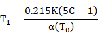
Once the value of a(T₀) is known, T₁ is calculated by:

The non-dimensional risk coefficient r is calculated by:

Finally, the modification factor of the spectrum u is calculated as a function of the damping by:

14.4.3                  Spectrum Calculation

The value of the ordinate of the spectrum a(T), represents the quotient of the absolute acceleration of an elastic linear oscillator (S_a) and the maximum acceleration of the movement applied on its basis (a):

 

The design spectrum S_d is given by:

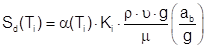
where:

 

 

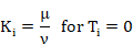
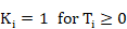
                                                    for T_i = 0

                                                      for T_i ³0

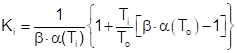     for 0 < T_i < T_o

 

If the last term of the previous formula is grouped into a factor y:

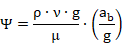
Then the following expression will be obtained:

A total of 20 values of the period T are calculated as specified below:

1.   The first 10 values for periods T_i between  and T₀ are calculated by:

where: i = 1 to 10

a.    If the spectrum type introduced with the SPTYPE parameter of the ~DEFSPEC command is linear, the ordinates of the spectrum a(T_i) are obtained with the following equation:

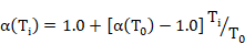
where: i = 1 to 10

b.    If the spectrum type is simplified, the ordinates of the spectrum are obtained by:

where: i = 1 to 10

2.   The remaining values of the period and of the ordinates of both spectrum types are calculated as follows:

a.    Values of the period:

where: i = 10 to 20

b.    Values of the ordinates of the spectrum, using the following equation:

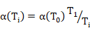
where: i = 10 to 20

Once the values of the period and the ordinates of the spectrum are calculated, the spectral accelerations are obtained for two orthogonal directions consisting of the global axes X and Y by applying:

For vertical movements, the ordinates of the spectrum will be reduced by a factor of 0.7.

 

14.5                 Spectrum Calculation according to NCSE-02

CivilFEM builds and defines the response spectrum in ANSYS from parameters through the following steps:

14.5.1                  Input data

The data required to define the response spectrum are input into the CivilFEM database with the ~DEFSPEC command.

The required data are listed below:

14.5.2                  Parameters for the Spectrum Definition

The ~DEFSPEC command calculates the parameters required for obtaining the elastic response spectrum. These parameters are input into the CivilFEM database through the following steps:

Once the data have been input, T_A and T_B are calculated by:

In addition, the amplification coefficient of soil S is calculated by:

 

 

 

Finally, the modification factor of the spectrum u is calculated as a function of the damping by:

14.5.3                  Spectrum Calculation

The value of the ordinate of the spectrum a(T) is defined as the quotient of the absolute acceleration of an elastic linear oscillator (S_a) and the maximum acceleration of the movement applied on its basis (a):

The design spectrum S_d is given by (Art. 3.6.2.2):

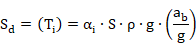
where:

S is the soil amplification factor

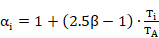                               if

              if

 is the normalized spectrum of elastic response (Art. 2.3):

       if

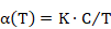                           if

                   if

A total of 20 values of the period T are calculated as specified below:

1.     The first 10 values for periods T_i between  and T_A are calculated by:

where: i = 1 to 10

a.     If the spectrum type entered with the SPTYPE parameter of the ~DEFSPEC command is linear, then the ordinates of the spectrum a(T_i) are obtained with the following equation:

where: i = 1 to 10

b.     If the spectrum type is simplified, then the ordinates of the spectrum a(T_i) are obtained by:

where: i = 1 to 10

2.     The remaining values of the period and of the ordinates of both spectrum types are calculated as follows:

a.    Values of the period:

where: i = 10 to 20

b.    Values of the ordinates of the spectrum, using the following equation:

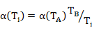
where: i = 10 to 20

Once the values of the period and the ordinates of the spectrum are calculated, the spectral accelerations are obtained for two orthogonal directions consisting of the X and Y global axes by applying:

 

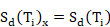
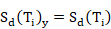
For vertical movements, the ordinates of the spectrum will be reduced by a factor of 0.7.

14.6                 Spectrum Calculation according to GB50011

CivilFEM builds and defines the response spectrum in ANSYS from parameters through the following steps:

14.6.1                  Input Data

The data required to define the response spectrum are input into the CivilFEM database with the ~DEFSPEC command.

The required data are listed below:

14.6.2                  Spectrum Parameters Definition

The command ~DEFSPEC calculates the parameters necessary for obtaining the response spectrum and introduces the data into the CivilFEM data base with the following procedure.

Firstly, the maximum value of the horizontal seismic influence factor is calculated with the data found in the table below:

Table 14.6‑1 Maximum value of the horizontal seismic influence factor: α_max

 

The characteristic period Tg is calculated from the soil and design group classifications through the following table:

 

Table 14.5‑2 Characteristic period of ground motion Tg

The following parameters are also calculated:

·         Declining power:

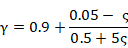
·         Inclined line ratio:

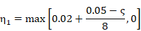
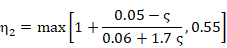
·         Adjusted ration of damping:

If the seismic factor and soil type correspond to values listed below, the response spectrum is displaced a distance of a period increment, following the table below:

 

Table 14.6‑3 T Increment

Otherwise, if the values do not correspond with those listed in the above, DT is taken as 0.05 if the seismic type is ‘RARE’ and the seismic factor is equal to 8 or 9.

14.6.3                  Spectrum Calculation

The horizontal response spectrum S_d(T) is defined as listed below:

 

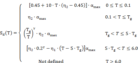
For vertical movements, the spectral Y coordinates are calculated proportional to the values corresponding to the horizontal movements’ spectrum.

 

 

 

 

 

 

 

 

 

 

 

 

 

 

 

 

 

 

 

 

 

 

14.7                 Spectrum Calculation according to GB50011-2010

CivilFEM builds and defines the response spectrum in ANSYS from parameters through the following steps:

14.7.1                  Input Data

The data required to define the response spectrum are input into the CivilFEM database with the ~DEFSPEC command.

The required data are listed below:

14.7.2                  Spectrum Parameters Definition

The command ~DEFSPEC calculates the parameters necessary for obtaining the response spectrum and introduces the data into the CivilFEM data base with the following procedure.

Firstly, the maximum value of the horizontal seismic influence factor is calculated with the data found in the table below:

Table 14.6‑1 Maximum value of the horizontal seismic influence factor: α_max

 

The characteristic period Tg is calculated from the soil and design group classifications through the following table:

 

Table 14.5‑2 Characteristic period of ground motion Tg

The following parameters are also calculated:

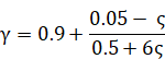
·         Declining power:

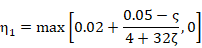
·         Inclined line ratio:

·         Adjusted ration of damping:

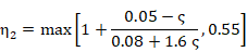
If the seismic factor and soil type correspond to values listed below, the response spectrum is displaced a distance of a period increment, following the table below:

 

Table 14.6‑3 T Increment

Otherwise, if the values do not correspond with those listed in the above, DT is taken as 0.05 if the seismic type is ‘RARE’ and the seismic factor is equal to 8 or 9.

14.7.3                  Spectrum Calculation

The horizontal response spectrum S_d(T) is defined as listed below:

 

For vertical movements, the spectral Y coordinates are calculated proportional to the values corresponding to the horizontal movements’ spectrum.

 

 

14.8                 Spectrum Calculation according to IT3274

CivilFEM builds and defines the response spectrum in ANSYS from parameters through the following steps:

14.8.1                  Input Data

The data required to define the response spectrum are input into the CivilFEM database with the ~DEFSPEC command.

The required data are listed below:

 

14.8.2                  Calculation of the Parameters for the Spectrum Definition

To define the horizontal and vertical response spectrum, the following parameters (which depend on the type of soil) are used:

 

Table 14.8‑1 Values which describe the horizontal response spectrum

 

Table 14.8‑2 Values which describe the vertical response spectrum

14.8.3                  Spectrum Calculation

14.8.3.1                   Elastic Spectrum

For the elastic horizontal response spectrum calculation, the following expressions are used:

Where:

 

For elastic vertical response spectrum calculation, the following expressions are used:

 

14.8.3.2                   Design Spectrum

For the elastic horizontal response spectrum calculation, the following expressions are used:

 

 

 

 

 

For elastic vertical response spectrum calculation, the following expressions are used:

 

 

 

14.9                 Spectrum Calculation according to AASHTO LRFD Bridge Design Specifications

CivilFEM builds and defines the response spectrum in ANSYS, from parameters through the following steps:

14.9.1                  Input Data

The data required to define the response spectrum are input into the CivilFEM database with the ~DEFSPEC command.

The required data are listed below:

 

14.9.2                  Calculation of the Parameters for the Spectrum Definition

To define the response spectrum, the Site Coefficient (which depends on the Soil Profile Type) is obtained from the following table:

 

Table 14.9‑1 Site coefficients

14.9.3                  Elastic Seismic Response Coefficient

For the elastic seismic response coefficient, the following expressions are used:

 

                                                          

 

For soil profiles III and IV:

             

    if              

 

14.9.4                  Elastic Response Spectrum

The horizontal elastic response spectrum is obtained from the elastic seismic response coefficient for each period, adjusted by the response modification factor R.

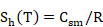
The vertical elastic response spectrum is obtained by multiplying the horizontal elastic response spectrum by the vertical ratio.

 

14.10           Spectrum Calculation according to EAK 2000

CivilFEM builds and defines the response spectrum in ANSYS from parameters through the following steps:

14.10.1              Input Data

The data required to define the response spectrum are input into the CivilFEM database with the ~DEFSPEC command.

The required data are listed below:

 

14.10.2              Calculation of the Parameters for the Spectrum Definition

To define the horizontal and vertical response spectrum, the following parameters are used:

 

Table 14.10‑1 Values which describe the response spectrum

 

Table 14.10‑2 Ground seismic acceleration: A = a·g

14.10.3              Spectrum Calculation

14.10.3.1                Elastic Spectrum

For the elastic horizontal response spectrum calculation, the following expressions are used:

 

Where:

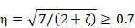
 (spectral amplification factor)

The elastic vertical response spectrum is derived from the elastic horizontal response spectrum by multiplying its ordinates by 0.70.

14.10.3.2                Design Spectrum

For the elastic horizontal response spectrum calculation, the following expressions are used:

For the elastic vertical response spectrum calculation, the following expressions are used:

where:

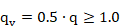
14.11           Spectrum Calculation according to CALTRANS Seismic Design Criteria

CivilFEM builds and defines the response spectrum in ANSYS from parameters through the following steps:

14.11.1              Input Data

The data required to define the response spectrum are input into the CivilFEM database with the ~DEFSPEC command.

The required data are listed below:

 

14.11.2              Spectrum Calculation

CALTRANS Seismic Design Criteria defines three response spectra for each soil profile type. Each of these three response spectra corresponds to a different earthquake magnitude.

The spectra defined by the CALTRANS Seismic Design Criteria (5% damping) are the following:

 

 

 

 

 

 

 

 

 

 

 

 

 

 

 

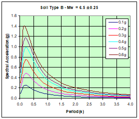
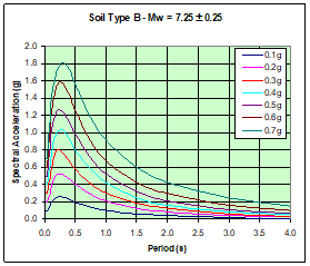
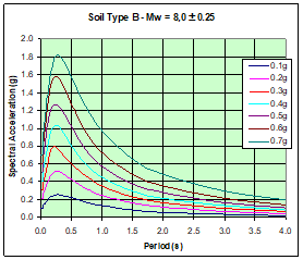
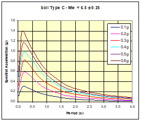
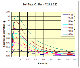
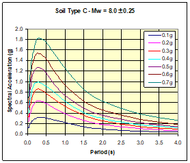
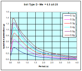
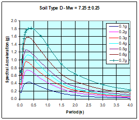
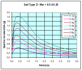
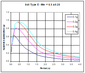
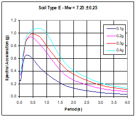
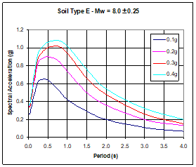
CivilFEM will interpolate the values of the predefined spectra to obtain the response spectrum which corresponds to the peak rock acceleration A·g.

The peak rock acceleration must be less than the maximum acceleration for an existing predefined spectrum (CivilFEM will not create higher spectra than the ones defined by CALTRANS). Therefore, the limits for A are:

 

 

Once the standard spectrum (ARS curve) is obtained, it will be modified if:

-          The structure is within 10 miles (15 km) of an active fault. In this case the spectral acceleration is magnified as follows:

o   Magnification is not required for T £ 0.5 s.

o   Increase by 20% for T ³ 1.0 s.

o   For 0.5 s < T < 1.0 s, the increase will be linear, with 0% for T = 0.5 s and 20% for T = 1.0 s.

-          The structure has a fundamental period of vibration T ³ 1.5 s and is on a deep soil site with a depth of alluvium ³ 250 feet (75 m). In this case the spectral acceleration is magnified as follows:

o   Magnification is not required for T £ 0.5 s.

o   Increase by 20% for T ³ 1.5 s.

o   For 0.5 s < T < 1.5 s, the increase will be linear, with 0% for T = 0.5 s and 20% for T = 1.5 s.

A reduction factor is applied to the 5% damped spectrum for damping 5% £ c £ 10%:

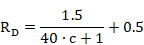
The vertical response spectrum is obtained by multiplying the horizontal response spectrum by the vertical ratio.

14.12           Spectrum Calculation according to the Uniform Building Code (1997)

CivilFEM builds and defines the response spectrum in ANSYS from parameters, through the following steps:

14.12.1              Input Data

The data required to define the response spectrum are input into the CivilFEM database with the ~DEFSPEC command.

The required data are listed below:

 

14.12.2              Calculation of the Parameters for the Spectrum Definition

To define the horizontal and vertical response spectrum, the following parameters are used:

 

Table 14.12‑1 Seismic zone Factor Z

 

Table 14.12‑2 Near source factor N_a

 

Table 14.12‑3 Near source factor N_v

 

Table 14.12‑4 Seismic Coefficient C_a for Design-basis earthquake

 

Table 14.12‑5 Seismic Coefficient C_v for Design-basis earthquake

 

Table 14.12‑6 Maximum capable earthquake response coefficient M_M

 

Table 14.12‑7 Seismic Coefficient C_a for maximum capable earthquake

 

Table 14.12‑8 Seismic Coefficient C_v for maximum capable earthquake

 

14.12.3              Spectrum Calculation

For the horizontal response spectrum calculation, the following expressions are used:

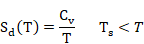
Where:

The vertical response spectrum is derived from the horizontal response spectrum by multiplying its ordinates by the vertical response factor (2/3 by default).

 

14.13           Spectrum Calculation according to PS 92

CivilFEM builds and defines the response spectrum in ANSYS, from parameters through the following steps:

14.13.1              Input Data

The data required to define the response spectrum are input in the CivilFEM database with the ~DEFSPEC command.

The required data are listed below:

 

14.13.2              Calculation of the Parameters for the Spectrum Definition

To define the response spectra, the following parameters (which depend on the type of soil) are used:

 

Table 14.13‑1 Values which describe the horizontal response spectrum

 

14.13.3              Spectrum Calculation

14.13.3.1                Elastic Spectrum

For the elastic horizontal response spectrum calculation, the following expressions are used:

 

 

 

Where:

The elastic vertical response spectrum is obtained from reducing the horizontal response spectrum by a factor of 0.7.

 

14.13.3.2                Design Spectrum

For the elastic horizontal response spectrum calculation, the following expressions are used:

 

 

 

The design vertical response spectrum is obtained by reducing the horizontal response spectrum by a factor of 0.7 if the soil type is S₀ or S₁. Otherwise, in addition to multiplying the spectrum by a factor, the descending branch will be replaced by the branch characteristic of a S₁ soil type.

 

14.14           Spectrum Calculation according to the Indian Standard 1893

CivilFEM builds and defines the response spectrum in ANSYS, from parameters through the following steps:

14.14.1              Input Data

The data required to define the response spectrum are input in the CivilFEM database with the ~DEFSPEC command.

The required data are listed below:

 

14.14.2              Calculation of the Parameters for the Spectrum Definition

To define the horizontal and vertical response spectrum, the following parameters are used:

 

Table 14.14‑1 Values which describe the response spectrum

 

Table 14.12‑2 Zone factor

 

Table 14.12‑3 Damping factor

 

14.14.3              Spectrum Calculation

14.14.3.1                Design Basis Spectrum

For the design basis horizontal response spectrum calculation, the following expressions are used:

 

 

 

   

For T £ T₁ the value of S_d will not be less than Z/2.

The design basis vertical response spectrum is derived from the elastic horizontal response spectrum, by multiplying its ordinates by 2/3.

14.14.3.2                Maximum considered earthquake spectrum

For the maximum considered earthquake horizontal response spectrum calculation, the following expressions are used:

 

 

 

For T £ T₁ the value of S_m will not be less than Z.

The maximum considered earthquake vertical response spectrum is derived from the maximum earthquake horizontal response spectrum by multiplying its ordinates by 2/3.

 

14.15           Modal Analysis of the Structure

The modes r and f_i and the natural vibration frequencies w_i of the structure are calculated by performing the modal analysis using the Subspace method (by default), Block Lanczos method or Householder reduced method (~MODLSOL command).

14.16           Modes Combination

Once the vibration modes are obtained by means of the ~CMBMOD command, they are combined for the indicated directions.

If the combination method is SRSS, for each one of the three directions (longitudinal, transversal and vertical), the result combination for the different vibration modes will be the square root of the sum of the squares of the variables. Once the significant vibration modes are combined in each one of the three directions (longitudinal, transversal and vertical), the obtained result is again combined by means of the square root of the sum of the squares.

For the remaining combination methods (CQC, DSUM, GRP and NRLSUM), it will only be possible to apply the spectrum as well as combine the vibration modes in one direction.

CivilFEM obtains a constant damping ratio from the spectrum data defined by the user. This constant damping ratio is required for the combination methods of CQC, DSUM and GRP.

The combination result will be stored in CivilFEM´s results file (file.RCV) with a Load Step number that continues from the last Load Step carried out. Therefore, in order to visualize this result, the ~CFSET command must be used. If this desired result pertains to any of the extracted vibration modes, the ANSYS SET command must be used since the vibration modes are stored in ANSYS´s results file (file.RST) as substeps belonging to the executed Load Step.

 

14.17           Push Over Analysis

14.17.1  Description

Push over analysis is a technique in which the model of a structure is subjected to a lateral load in a predetermined way. The intensity of the load is increased successively as a function of certain multiplication factor l.

During the “l increase – analysis” process, the structure starts with an initially elastic behavior (linear or not linear, depending on the material). It then goes through different weakening phases due to yielding and other local effects until it reaches collapse.

Depending on observations of the behavior of the structure, structural deficiencies can be deducted from each calculation phase. These deductions lead to a manual iterative analysis, once these deficiencies are corrected (Retrofit Analysis).

This process is especially suited for building type structures.

 

14.17.2  Structure Capacity

The following figure shows a structure (in this case a lighthouse) subjected to a vertical load W (self weight + other loads) and to a lateral wind load.

 

 

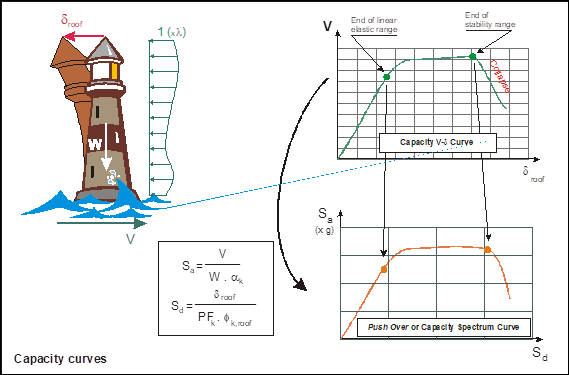
The lateral wind load is subjected with an intensity determined by the parameter l; in this case, l represents the value of the pressure at the top of the structure.  As a result of this wind load, the structure suffers a deformation that is measured by the displacement of the highest point:

And by a horizontal reaction (wind direction) at the base:

V(l)

By representing the pair of values d_roof and V on a Cartesian chart, the capacity curve or V-d curve can be obtained. From this curve, critical points can be observed such as the yield point or the point that signifies the start of collapse.

Following, a modal analysis of the structure is performed and the vibration mode k with the highest participation factor PF is obtained (typically k=1, except if local modes are present). The following factors are defined as:

 

 

 

 

In these expressions, f_ik is the i-th component of the vibration mode k, and m_i is the mass that corresponds to the associated degree of freedom.

Vibration modes are normalized, so that:

 

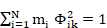  (N = total number of degrees of freedom)

 

Therefore, the previous expressions can be simplified:

 

 

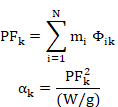
To perform the Push Over analysis, variables are converted from the d_roof –V diagram to the S_d – S_a diagram, referred to as the Acceleration-Displacement Response Spectrum or the ADRS.

The new variable relationship is as follows:

 

 

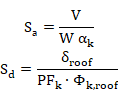
Both curves are found in the previous figure.

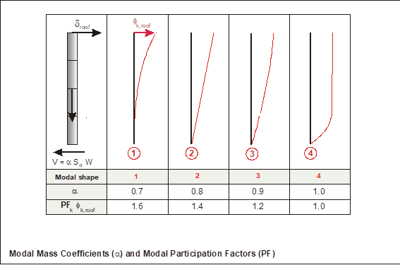
The following figure presents typical values of the previously defined parameters for different shapes of the dominant vibration mode k.

 

 

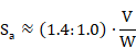
Therefore:

 

14.17.3  Seismic Response Spectra

Response spectra are commonly defined as accelerations (S_a), pseudovelocities (S_v) or displacements (S_d) versus the vibration period T.

Between these four magnitudes, the following relationships can be defined:

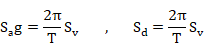
when S_a is expressed as fractions of g.

Eliminating S_v from the previous expressions, the following equation is obtained:

This equation defines the relationship between the acceleration and the displacements spectra.

The following figure displays the acceleration spectra in the standard format (T,S_a) as well as the derived format (S_d, S_a), otherwise known as the ADSR.

 

 

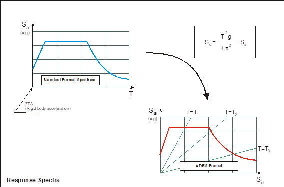
For the lines of the ADRS format:

S_d/S_a = c, (constant)

Therefore, these lines that pass through the origin represent the locations of equal vibration period on this plane.

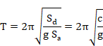
When the value of T decreases, the stiffness of the structure increases.  For example, the value of S_a for T = 0, is known as the zero period acceleration or ZPA. Therefore, the value of:

for these straight lines is a measure of the stiffness, as described in later sections.

 

14.17.4  Push Over Analysis

The Capacity Structure Curve, CSC, is obtained from a nonlinear analysis by increasing the loads by a factor l.  This curve is then superimposed onto the ADRS spectrum (or Demand Spectrum Curve, DSC), as seen below:

 

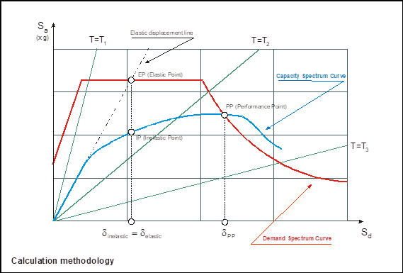
If a structure remains elastic during the entire load process, the intersection point of the CSC and DSC curves (capacity and demand), or the Performance Point (PP), represents the equilibrium situation. Therefore, d_pp is the deformation when the earthquake acts on the structure.

 

However, in general, a structure does not remain in its elastic regime during the entire process; therefore, some authors prefer to consider the inelastic point IP as a working point in the presence of an earthquake, as shown in the figure above.  This is equivalent to assuming, with respect to displacements, the structure will maintain its elastic behavior until it intersects the demand curve, with respect to displacements.

 

14.17.5  Retrofit

During the loading process, local yielding phenomena cause the structure to weaken, but not to collapse. This weakening effect is represented by the curve approaching the horizontal.

In the following figure, a beam structure is subjected to an action that is proportionally increased by a multiplication factor l_i (l_i > l_j if i > j).

 

 

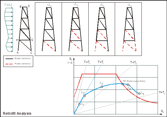
For values l < l₂, the structure remains elastic (and in this case linear) with a stiffness determined by the line corresponding to the period T = T_I. When the value l₂ is reached, the diagonal bar PC yields, and the structure is weakened until it reaches a dangerous situation at l = l₄. At this moment the bars AP and PC have yielded. Collapse is achieved at l = l₅ with the total yield of the lower level of the structure.

The individual analyses of the state of the structure at each of the phases (scenarios) allow the engineer to determine which sections require reinforcement to obtain a more appropriate capacity curve.

 

14.17.6  Procedure

The Push Over analysis follows the steps below:

 

1. Creation of the finite element model.
2. Definition of the response spectrum and modal analysis.
3. Definition of the vertical loads which remain constant during the process. They must be defined as masses.
4. Definition of the horizontal loads, which will be increased by the l factor. These loads are stored in a load state file (~CFLSWRT command).
5. Definition of a variation range for the l parameter: l_i, l_f and the increment Dl (~PUSHDEF command)
6. Selection of the predominant mode (~PUSHMOD command).
7. Analysis of the structure subjected to the loads defined in steps 3 and 4, varying l as established in step 5 (~PUSHSLV command).
8. Calculation of the CSC curve.
9. Calculation of the DSC curve.
10. Calculation of the IP and PP points.
11. Graphical representation of a scenario selected by the user (through Sd or l), displaying the proximity to the yield state with colors (~RETROFT command).

The results can be listed using the ~PUSHLST command. The obtained curves can be seen through the graphical interface.

 

14.18           Seismic Safety Margin

14.18.1  Description

Seismic margin methodology provides a quantification of a nuclear power plant’s ability to withstand a site specific earthquake design motion and enables a safely shut down if capacity is exceeded.

The goal is to quantify this capability and develop practical methods of assessing nuclear plant seismic margins.

For this reason, interest has developed in defining the margin above the Safe Shutdown Earthquake (SSE) that exists in operating plants. While defining this margin is a desirable goal, it is more practical to select an earthquake level for which the ability to safely shut the plant down can be demostrated with high confidence in a cost-effective manner. Only those systems and components which are required to bring a plant to, and maintain, a safe shutdown condition following the seismic event need to be examined. The earthquake level against which the plant is evaluated is commonly referred as the Seismic Margin Earthquake (SME).

Although highly unlikely, it is possible for a nuclear power plant to be subjected to earthquake ground motion greater than that for which the plant was designed. For this reason there is an interest in defining the margin above the SSE that exists in operating plants, an upper limit of seismic capacity which would render components inoperable if exceeded.

The Electric Power Research Institute (EPRI) and the Nuclear Regulatory Comission provide methods to asses seismic safety margin by either utilizing results of a Seismic Probabilistic Risk Assesment (SPRA) or by conducting a deterministic Seismic Margin Assesment (SMA).

A third approach (EPRI NP 6041) is recommended and is the one implemented in CivilFEM. This approach reviews the plant against a specific earthquake level an determine whether the plant has a high confidence of low probability of failure for SME. If less than SME, then calculate the plant High Confidence Low Probability of Failure (HCLPF) capacity.

 

14.18.2   High Confidence of Low Probability of Failure

HCLPF is defined as high confidence of a low probability of failure and can also be interpreted as approximately a 95% confidence of about 5% (or less) probability of failure.

The deterministic approach and procedures for calculating the HCLPF in EPRI NP 6041 uses the Conservative Deterministic Failure Margin (CFDM) method.

Conservative Deterministic Failure Margin (CDFM) approach will be used to compute the SME capacity of structures and components and intends to achieve the following:

1.    For the specified SME, the elastic computed response (SME Demand) of structures and components mounted thereon should be defined at the 84% non-exceedance probability.

2.    Capacities for most components should be defined at about the 98% exceedance probability so that even if the SME demand slightly exceeds this CDFM capacity by more than a permissible conservately specified inelastic energy absorption capability, there will result a very low probability of failure.

3.    Inelastic distortion associated with Demand/Capacity ratio greater than unity is permissible. The permissible level of inelastic distortion should be specified at about the 5% failure probability level.

4.    Finally: Seismic Demand/Capacity ≤ F_μ, where F_μ is the inelastic energy absorption factor.

In a SMA calculation to compute the seismic capacity, a Reference seismic Margin Earthquake level SME_R is defined and then a linear elastic seismic demand D_S for this earthquake. The capacity/demand ratio for elastic response is:

 

 

Similarly, for a permissible level of inelastic response, the inelastic capacity/demand ratio is:

 

Where:

 

 

The CDFM seismic margin earthquake level SME exceeds SME_R when (C/D)_I ratio exceeds unity.

However, (C/D)_I ratio does not define the scale factor by which Reference seismic Margin Earthquake (for example SME_R=0.3g) level may be scaled to obtain the CDFM SME level.

The scale factors (FS)_E and (FS)_I by which the SME_R can be scaled for elastic and permissible inelastic response are given by:

 

 

Then capacity level of Seismic Margin Earthquake (SME) according to Conservative Deterministic Failure Margin (CDFM) is:

 

 

14.18.2.1                Structure response (demand) calculation

The structure demand will be the forces and moments on each finite element end which are D_NS  (non seismic combination) and D_S (seismic combination) shown in scale factors (FS)_E (FS)_I formulas.

14.18.2.2                Structural capacity calculation

The structural capacity will be calculated taking into account the following:

 

1.    Material strengths: If actual material properties area available (obtained with sufficient test data), 95% exceedance probability strengths will be used. Otherwise, code specified minimum strengths will be used.

These material strengths and properties will be set in the finite element model before solving the loads cases and combinations.

 

2.    Static Capacity: the static capacity will be calculated taking into account code specifications and material strengths calculated in above point, performed in all the element ends of the finite element model. 

For buckling capacity, whole member length and properties will be considered.

 

3.    Inelastic Energy Absorption Factor: nearly all structures and components exhibit at least some ductility (i.e, ability to strain beyond the elastic limit) before failure. Because of the limited energy content ans oscillatory nature of earthquake ground motion, this ductility is highly beneficial in increasing the seismic margin against failure for structures and components. The inelastic energy absorption factor Fμ, represents the ratio of SME at which certain ductility μ is reached to the earthquake level for which a limit state would be predicted by linear elastic analysis.
These factors will be taken as input data from either beam cross sections code properties (~SECMDF command) or shell vertices (~SHLMDF command).

 

4.    Reduction in capacity due to concurrent seismic loads, ΔC_S. For example, the shear capacity of a shear wall under horizontal spectra is reduced by the seismically induced vertical tensile load due to vertical spectra. Since the seismic loads scenarios are a result of SRSS combination of the considered spectra in each of the three directions of space and also reversal signs for the seismic forces and moments, the concurrent seismic loads effects are all taken into account with a higher accuracy, therefore ΔC_S is considered when calculating the section capacity.

14.18.3              Available codes

Structure capacity for seismic design will be calculated according to the provisions of the following available codes for reinforced concrete structures (beam and shell elements):

·         Axial and bending check: all available codes.

·         Shear and torsion check: Eurocode 2 (ENV 1992-1-1:1991 and EN 1992-1-1:2004/AC:2008); ACI 349-01.

·         In-plane shear check: ACI 349-01.

For structural steel codes: Eurocode 3 (EN 1993-1-1:2005); ANSI/AISC N690-06 (both LRFD and ASD specifications).

A full description of code cheking processes is located in its corresponding chapter within CivilFEM Theory Manual.

14.18.4              Seismic margin check procedure

For the Structure Demand Calculation (D_NS and D_S), the finite element model will be solved by performing static analysis for the non-seismic loads and a response spectrum analysis for the seismic demand.

The structural capacity C_S and the scale factors (FS)_E (FS)_I will be calculated by CivilFEM following the specifications of any of the implemented codes but two different RCV files (for seismic and non-seismic load combinations) must be defined before seismic margin check is performed.

The general procedure applicable for all seismic margin checks is described as follows:

 

1.    Define geometry and mesh model as usual.

2.    To consider ductility add corresponding inelastic energy absorption factors in cross sections or/and shell vertices.

3.    Solve the different load combinations, one for seismic and other (s) for non-seismic loads using a different jobname for each RCV file.

4.    Indicate which the current seismic combination is with ~CFFILE2 command.

5.    Check reinforced concrete structures with ~HCLPFCN command or check steel structures with ~HCLPFST command.

6.    Review seismic margin results for reinforced concrete with ~PLHCLPF, ~PRHCLPF, ~IDHCLPF, ~PLSHCLP, ~PRSHCLP commands.

7.    Review seismic margin results for structural steel with ~HCLPFST, ~PLSHCLP and ~PRSHCLP commands.

 

14.18.4.1                Axial + bending check in reinforced concrete

Seismic margin check process of reinforced concrete beams and shells subjected to axial force plus bending moment according to code is based on the 2D interaction diagram of the considered cross section or shell vertex instead of using equations 14.18.3 and 14.18.4. Demand and capacity are given by a vector (N,M) corresponding to ultimate strength states determined through the pivot diagram.

The construction of the interaction diagram is described in chapters 11-A.3, 11-A.4 and 13-1.3 but with the following differences:

 

1.    Non-seismic demand, D_NS, is obtained from nonseismic (static) results file (axial force and bending moment).

2.    Seismic demand, D_S, is obtained from seismic (spectral) results file (axial force and bending moment).

3.    Total demand is the sum of non-seismic and seismic demand: D_T = D_NS + D_NS

4.    Center of interaction diagram is the non-seismic demand: (NX,MY) or (NX,MZ) in beam cross sections and (TX,MX) or (TY,MY) in shell vertices.

5.    Ultimate axial force and bending moment (Nu,Mu) are actually the deterministic seismic capacity C_S.

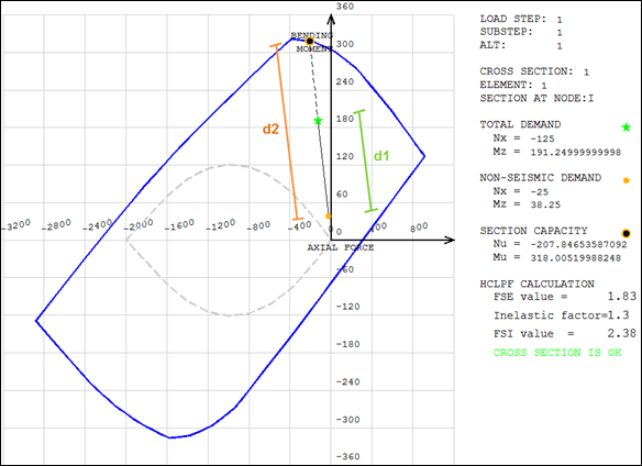
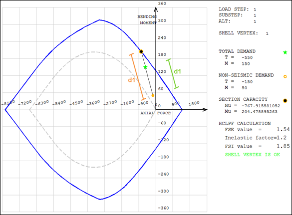
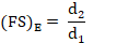
6.    Scale factor for elastic response (FS)_E, is defined as the ratio of two distances. As shown in figures below, d1 is the distance from the center of the interaction diagram to the point representing the total demand and d2 is the distance from the center to the point representing the ultimate axial force and bending moment (seismic capacity).

7.    Scale factor for permissible inelastic response (FS)_I, is computed by multiplying scale factor for elastic response (FS)_E  by the inelastic energy absorption factor.

If (FS)_I exceeds unity (1.00) then the cross section or shell vertex is considered with a safe seismic margin capacity level.

For beam cross sections:

 

For shell vertices:

14.18.4.2                Other checks

The process of seismic margin check consists of obtaining the factor such that criterion check of non-seismic loads and factorized seismic loads is equal to unity.

 

 

Where:

Dns: Nonseismic demand

Ds: Seismic demand

 

The procedure to calculate the mentioned criterion value is described in corresponding chapters of CivilFEM Theory Manual for each code and check types.

To obtain the value of FSE factor, CivilFEM takes into account the following considerations:

• Values of (0.0-1.0) interval are computed, if none of these values within that range make criterion value greater than unity then CivilFEM returns last criterion value checked.
• If criterion of non-seismic loads is greater than unity then CivilFEM returns -1.0 as FSE result and criterion check for non-seismic loads.

Scale factor for permissible inelastic response (FS)_I, is computed by multiplying scale factor for elastic response (FS)_E  by the inelastic energy absorption factor.

 

If (FS)_I exceeds unity (1.00) then the cross section or shell vertex is considered with a safe seismic margin capacity level.

Note: For Eurocode (EN 1993-1-1:2005) seismic margin is not calculated if:

• Any of its ends is in compression for seismic loads and check type is tension.
• Any of its ends is in tension for seismic loads and check type is compression, compression buckling or flexural and compression buckling.