

Chapter
18-A
Bridge and Civil Non Linearities Module (Part I)
18-A.1 Introduction
A frequent circumstance in engineering and particularly in civil engineering is that the transverse section of a member suffers variations due to sources so variable as the following:
- Change in geometry due to construction process. It can be the case of deep beams and composite beams for bridge decks.
- Change in the material properties, hardening, aging, shrinkage or rheological phenomena.
- Loss of resistant properties due to plasticizing or partial cracking.
With the purpose of giving answers to these problems, CivilFEM includes the non linear beams module.
It's use allows the consideration of the real stress-strain law (not linear) of the material, introducing, for that purpose, changes in the parameters managed by ANSYS during the successive calculation iterations. These parameters are the real constants of the elements and the adopted procedure will be seen with more detail in the following sections.
CivilFEM controls, during the whole process, the current calculation time (see command ~ACTTIME) and the activation time of each material (see command ~CFMP), obtaining this way the age of each material. This porcedure, allows the use for each calculation time, of a different stress-strain law that can be linear or non linear.
Besides solving beam non-linear analysis, the bridge and civil non-linearities module includes an utility that allows performing evolutive calculations of cross sections.
The main objective of this capability is to take advantage of the evolutive characteristics of the CivilFEM materials contained in the beam cross sections, with birth and variation of the material time dependent properties. In order to use this capability, the utility in CivilFEM for non-linear analysis of beams described on section 18.3 must be deactivated since an elastic and linear behaviour of each of the materials forming the cross section is assumed.
18-A.2 Types of Elements for Non-linear Analyses
The different type of elements supported by CivilFEM for the concrete creep models are the following:
- Step by step method
|
Beams |
LINK180, BEAM188, BEAM189 |
|
Shells |
SHELL181, SHELL281 |
|
2D Solids |
PLANE182, PLANE183 |
|
3D Solids |
SOLID185, SOLID186, SOLID187 |
- Effective modulus method
All the ANSYS structural elements.
The elements supported by CivilFEM for the concrete shrinkage models are all the ANSYS Structural elements except:
- All PIPE elements.
- SHELL91, SHELL181, SHELL281, SOLID191.
- It can only be used on SHELL99 and SOLID46 elements if KEYOPT(2) = 0 or 1.
The different type of elements supported by CivilFEM for the non-linear analysis of beams are the following:
|
2D Bars |
LINK1 |
|
3D Bars |
LINK8, LINK10 |
|
Tapered 3D Beams |
BEAM44 |
|
Tapered 2D Beams |
BEAM54 |
The rest of elements are not taken into account by the non linear module, introducing them in the analysis in the conventional way followed by ANSYS.
18-A.3 CivilFEM Evolutive Analysis of Beams
18-A.3.1 Introduction and Objective
The main objective of this capability is to take advantage of the evolutive characteristics of the CivilFEM materials contained in the beam cross sections, with birth and variation of the material time dependent properties.
This problem may be solved with relative easiness, using ANSYS birth and death of elements, but it is then necessary to use a different element type for each defined material conforming the cross section as well as the definition of each cross section and offsets.
18-A.3.2 General Considerations
In order to use this capability, the utility in CivilFEM for non-linear analysis of beams must not be activated (an elastic and linear behaviour of each of the materials forming the cross section is assumed).
The objective is valid only for small strains, that is, if small strains are negligible compared to the initial element length.
Cross sections in CivilFEM for evolutive analysis purposes may only contain up to 100 different materials.
The sections should have the parameter ASEC=8. The evolutive analysis needs the section properties to be homogenized according to the elasticity module of the materials that compose the section.
18-A.3.3 Approach
The main problem comes from the birth of the materials in the cross section when the element is deformed. These materials, when born, have zero strains and therefore they modify the movement of the element with regards to the applied loads.
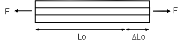
A clear example of this phenomenon is a beam submitted to axial forces and formed by 2 different materials, one of which is born after the first one has being loaded.
If Lo is the initial element length, in which only the first material has born, if the element is loaded with an axial force, an elastic strain deformation appears:
 |
If in this precise moment the second material is born, the axial force is still supported by the first material, therefore stresses and strains acting on this material must remain. As well as the total movement of the element. Nevertheless, stresses and strains in the second material must be zero.
 |
When the applied loads change, movements, stresses and strains in the different materials will not coincide with the ones obtained when considering the stiffness of both materials. Considering the particular case of no loads acting on the beam:
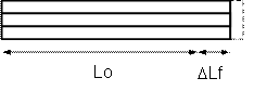 |
we can obtain a residual strain on the element not loaded, as well as an auto-equilibrated stress system acting on each material forming the cross section:
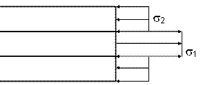 |
The solution of this problem with CivilFEM beams consists in considering the imposed strains without modification of the stress field, as well as the correction of the strains and stresses in each material.
18-A.3.4 Imposed Strains
From the previous section it is clear that it is necessary to impose on each element the strain necessary to reproduce the real movement of the structure’s elements, considering the birth of the different materials conforming the cross section.
These impose strains are applied automatically by the software as temperature increments on each elements.
18-A.3.4.1 Link Elements
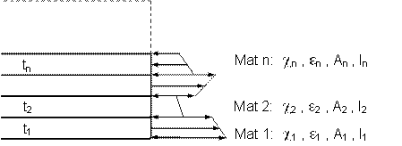
In the case of Link type elements, considering a section in a generic situation in which the different materials 1 to n have born at different times:
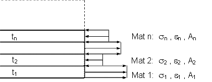 |
The areas indicated above are the areas corresponding to the homogenized modulus of elasticity used in the analysis.
The temperature increment that will be applied is the following:
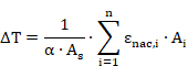
Where:
a Material thermal expansion coefficient to which the cross section is homogenized
As Homogenized area of the actual cross section (of the born materials)
Ai Homogenized area of material i
enac,i Element strain when material i is born.
18-A.3.4.2 2D Beam element type
On elements supporting bending forces with respect to one axis as well as axial loads, the strains from a particular will be a function of the strain e of a particular point and the curvature c.
 |
The temperature increments to be applied in the top and bottom fiber are obtained solving the following system of equations:


Where:
DTsup Temperature increment in the top fiber
DTinf Temperature increment in the bottom fiber
hsup Distance from the COG to the top fiber (of the born materials)
hinf Distance from the COG to the bottom fiber (of the born materials)
hs Thickness of the cross section (of the born materials)
a Material thermal expansion coefficient to which the cross section is homogenized
As Homogenized area of the cross section (of the born materials)
Is Homogenized inertia of the cross section (of the born materials)
Ai Homogenized area of material i
Ii Inertia of material i.
di Distance from the COG of the actual cross section to the COG of the considered material
enac,i Real strain of material i measured from its birth in the COG of the material
cnac,i Real curvature of material i measured from its birth
18-A.3.4.3 3D Beam element type
In this case (elements, apart from axial forces, can sustained flexural forces in two directions), strains of a particular material are a function of the strain e of a particular point and curvatures cy and cz.
In 3D beam elements, ANSYS allows to introduce, at each element end, four temperatures (from now on, when referring to temperatures, it will be understood that these are increments of temperatures):
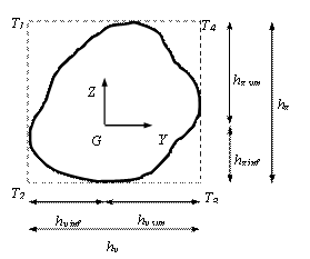 |
 In this case, the
axial strain is calculated taking the mean value of the four temperatures, and
the curvature as the mean value of the temperatures in the top and bottom
fibers in each direction.
In this case, the
axial strain is calculated taking the mean value of the four temperatures, and
the curvature as the mean value of the temperatures in the top and bottom
fibers in each direction.
Expressing the strains as a function of the corner temperatures:
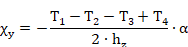
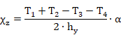

In this case, the applied temperature increments are obtained by solving the following system of 3 equations and 4 unknowns, considering a value of zero for the temperature increment T4.

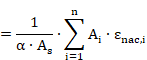


18-A.3.5 Real stress and strain analysis
In the previous sections, the temperature increments to be imposed in order to reproduce the structure real movement have been calculated. Real strains are calculated taking into account the birth strains of each material:
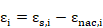
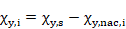
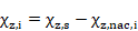
Where:
ei Real material i strain measured from its birth in the COG of the material
es,i Strain of COG of material i (Elastic plus thermal)
enac,i Strain from birth of the COG of material i
cy,i Real curvature of material i from Y axis measured from its birth
cy,s Y axis curvature of the section
cy,nac,i Y axis curvature of birth of material i
cy,i Real curvature from Z axis of material i measured from its birth
cz,s Z axis curvature of the section
cz,nac,i Z axis curvature of birth of material i
The strain at any fiber of the material i is:

YG,i Y coordinate of material i COG
ZG,i Z coordinate of material i COG
The elastic stresses are obtained by multiplying the strain by the real modulus of elasticity of the corresponding material:

18-A.3.6 Considerations with respect to user defined temperatures
Temperature increments introduced by CivilFEM are transparent to the user. These increments are added automatically to the existing ones introduced by the user, and subtracted after the solution.
The total thermal strains can be decomposed as:

where:
 Total
thermal strains
Total
thermal strains
 Strains due to the
temperature increments introduced by the user
Strains due to the
temperature increments introduced by the user
 Thermal strains introduced
by CivilFEM for taking into account the evolutive process.
Thermal strains introduced
by CivilFEM for taking into account the evolutive process.
The thermal strains on each fiber due to a temperature increment introduced by the user are:

being:

where:
 Thermal
strains at COG
Thermal
strains at COG

 Direct
thermal strain
Direct
thermal strain
 Thermal
strain in the Z top fiber
Thermal
strain in the Z top fiber
 Thermal
strain in the Z bottom fiber
Thermal
strain in the Z bottom fiber
 Thermal
strain in the Y top fiber
Thermal
strain in the Y top fiber
 Thermal
strain in the Y bottom fiber
Thermal
strain in the Y bottom fiber
hz Thickness of cross section with respect to Z axis
hy Thickness of cross section with respect to Y axis
zG Coordinate of COG with respect to Z axis
yG Coordinate of COG with respect to Y axis
On the other hand, the thermal strains introduce by CivilFEM are:

Where the strain of the COG and curvatures correspond to the ones calculated on section 18.12.3:
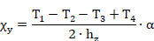
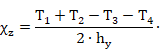


18-A.3.7 Non linear analysis
In all the previous sections, an elastic and linear behavior of all the materials conforming the cross section has been considered. Analysis considering the material non-linear behavior can produce erroneous results.
18-A.3.8 Materials with time dependent modulus of elasticity
CivilFEM contemplates the possibility of considering the plasticity module as a function of time. As when the materials are born in the cross section, an increment of the modulus of elasticity of the materials conforming the cross section forces the introduction of new temperature increments that will reproduce the movements and will correct the stresses on each material.
To simulate the process, it is necessary to take into account the history of the changes of the modulus of elasticity experimented by the materials. This is done by updating on each load step the material birth strain.
This update of a particular material birth strain that increments its modulus of elasticity from Ei,1 to Ei,2 is carried out using the following formula:
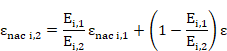
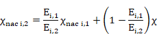
where:
enaci,1 Birth strain of COG of material i at instant 1
enaci,2 Birth strain of COG of material i at instant 2
cnaci,1 Real curvature of material i measured from its birth at instant 1
cnaci,2 Real curvature of material i measured from its birth at instant 2
e Strain of structure’s COG when the modulus of elasticity changes
c Curvature of section when the modulus of elasticity changes
Ei,1 Elastic modulus of the material i at instant 1
Ei,2 Elastic modulus of the material i at instant 2
18-A.3.9 Deleting or reducing the elasticity modulus of a material
In the previous formulation, it has always been assumed that new materials had born or that the modulus of elasticity had been increased. This assumption implies for a particular instant of time, the birth of a material without strain and therefore without tension.
In the event of materials being removed or modulus of elasticity being decreased, for the results to be correct these situations only make sense for materials without stresses.
18-A.3.10 Temporary file
During the execution of the evolutive analysis, CivilFEM creates 2 temporary files with extensions EVL and EVLI which are automatically removed when the /SOLU processor is exited.
18-A.3.11 Results output
Stresses and strains results need to be postprocess using CivilFEM utilities (see commands ~PLCSSTR and ~PLLSSTR). Evolutive analysis results may be combined using CivilFEM combination utilities.
18-A.4 Creep and Shrinkage
18-A.4.1 Introduction
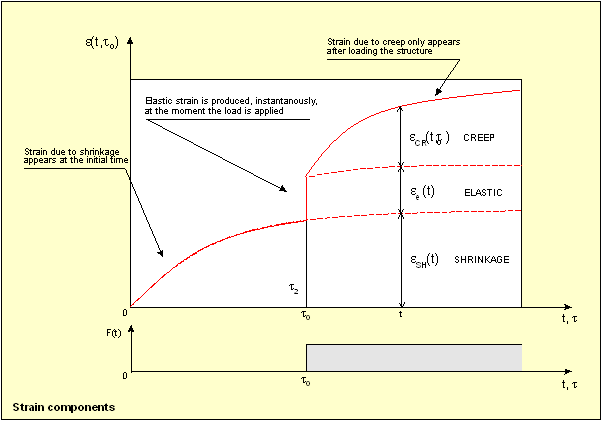
Shrinkage and creep are long term time-dependent effects and can cause strains and displacements that can change forces, stresses, reactions or the prestress load which the structure is subjected to.
Shrinkage is an unloaded time-dependent deformation, while creep is an under load time-dependent deformation. Although both concepts are two aspects of a single complex physical phenomenon, based on the reological behavior of concrete, they should be considered as independent and studied separately.
Time-dependent deformation of a concrete member under constant stress (ignoring thermal expansion) is computed as:

where:
|
|
Instant elastic strain |
|
|
Creep strain at age t |
|
|
Shrinkage strain at age t |


Elastic and creep strains are stress-dependent and are usually considered together and shrinkage strain separately.
One of the hypothesis in the study of creep is linearity, means that strain is proportional to stress:
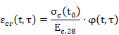
where:
|
|
Creep strain at time t under a constant stress applied at t |
|
|
Constant stress applied at time t |
|
|
Elasticity modulus at 28 days |
|
|
Creep coefficient |


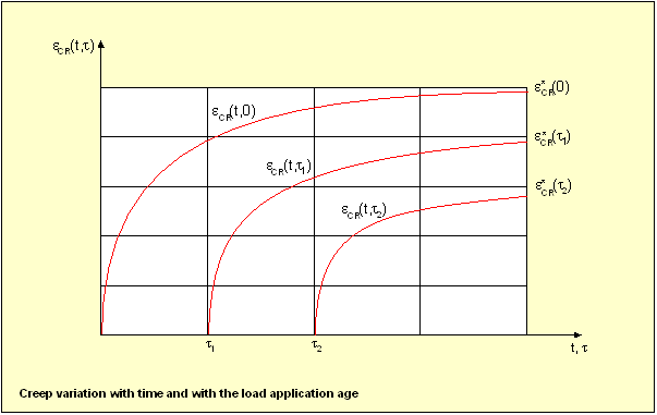
Therefore, stress-dependent strain may be estimated from:

|
|
Elasticity modulus at loading age t |
|
|
Creep function |


Validity of linearity hypothesis is experimentally confirmed for initial stresses not greater than 40% of concrete mean compressive strength.
Another hypothesis commonly accepted is the superposition principle, which says that the strain produced in concrete at any time t by any increase of stress applied in time t, is independent from any increase of stress produced before or after t.
So, defining  as
the strain produced by a load applied in t1 and
as
the strain produced by a load applied in t1 and  as
the strain produced in a time t2 (t2 > t1), as result of both loads:
as
the strain produced in a time t2 (t2 > t1), as result of both loads:

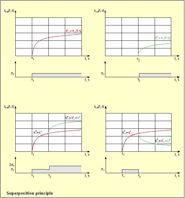
Creep strains are, therefore, addable, so the total strain of concrete for a history of variable loads should be:
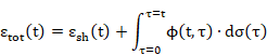
|
|
Total strain at time t |
|
|
Shrinkage strain |
|
|
Creep function |
|
|
Stress variation at time t |


18-A.4.1.1 Shrinkage analysis method
Shrinkage in CivilFEM is computed from shrinkage strain curves defined in concrete materials. This curves are calculated from the available codes in the program or can be defined point by point.
Shrinkage strains will be computed in all materials activated with this option. They are introduced in the model by temperature increments and calculated from strain and thermal expansion coefficient of the material.
Shrinkage strains are related with thermal strains,therefore, temperature increments must not be applied to elements which have shrinkage activated in associated material.
For a correct evaluation of time-dependent properties, ANSYS time defined with command TIME, must coincide with active time of CivilFEM defined with command ~ACTTIME.
18-A.4.1.2 Creep analysis methods
In CivilFEM actual version are implemented the following methods:
a) Step by step method
b) Effective modulus method
The activation of one or the other method is only applied on concrete materials defined in the model. There is no inconvenience on working with concrete materials with different creep method evaluation or with concrete materials without this phenomenon.
a) Step by step method
For the calculation of the integral explained in the previous chapter (analysis in time of a structure subjected to creep), CivilFEM uses the step by step standard method.
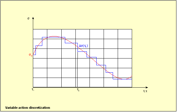
In the step by step method the time is divided into a series of intervals, so that in each of the intervals the equilibrium and compatibility conditions of the structure are satisfied.
To do so, time t is divided into times series t0, t1, t2, ..., tk. Strain is computed as follows:

The solution procedure of CivilFEM employs a non linear calculation with automatic time discretization: the time steps, corresponding to ‘load steps’ and ‘substeps’, are chosen to follow the evolution of loads and model geometry.
Strain increments produced by creep are computed from creep coefficients defined in the material and from stress increments produced during time discretization:

This creep strains are introduced in the model using ANSYS Creep (routine UserCreep is programmed for this case, which uses an implicit time integration algorithm).
Is possible as well, to take into account an aging coefficient so creep strains are computed as follows:
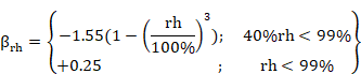
Where t1 is the application time of first load.
If a null value is introduced for aging coefficient, the program takes internally:
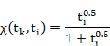
As same as shrinkage, For a correct evaluation of time-dependent properties, ANSYS time defined with command TIME, must coincide with active time of CivilFEM defined with command ~ACTTIME.
b) Effective modulus method
This method consists using a elasticity modulus called effective modulus which takes into account the additional strain caused by phenomenon of creep
The effective modulus is calculated by the following expression:
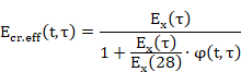
|
|
Material age at the moment of the calculation |
|
|
Concrete age at the moment of the loads application |
|
|
Elasticity modulus at 28 days |
|
|
Elasticity modulus at the moment of the loads application |
|
|
Creep coefficient |


The concrete age at the moment of the load application is calculated as the difference between the load application time, TAppLoad (see ~CFMP command) and the material activation time, Tact (see ~CFMP command).

This simplified method needs only one load step for each time to be solved, so this method is much faster that step by step method.
Under this method, the creep strain only depends on the current state of stresses that’s why it’s independent of the previous load history. This method provides accurate results for concrete stresses almost constant in time.
This method is based on the substitution of the material elasticity modulus by an effective modulus so it isn’t possible to determine the creep strain independent to the elastic strain so the final elastic strain will be the combination of these.
18-A.4.2 EHE Spanish Code
18-A.4.2.1 Creep
In this code the creep coefficient may be calculated from:

Where, j0 is the notional creep coefficient and bc is a coefficient to describe the development of creep with time after loading, t is the age of concrete in days at the considered moment and t0 the age of concrete at loading in days:

where:
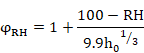
is a factor to allow for the effect of relative humidity on the notional creep coefficient.
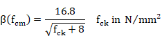
is a factor to allow for the effect of concrete strength on the notional creep coefficient and fck is the characteristic compressive strength.
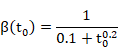
is a factor to allow for the effect of concrete age at loading on the notional creep coefficient.
 is the notional size of member in millimetres, where Ac is
the cross section and u is the perimeter of the member in contact with
the atmosphere.
is the notional size of member in millimetres, where Ac is
the cross section and u is the perimeter of the member in contact with
the atmosphere.
The coefficient for the development of creep with time may be estimated from:
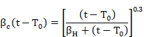

Where (t-t0 ) is the non-adjusted duration of loading in days and bH is a coefficient depending on the relative humidity (RH in %) and the notional member size h0 (mm).
18-A.4.2.2 Shrinkage
The shrinkage or swelling strains may be calculated from:

where:
|
esh0 |
Notional shrinkage coefficient |
|
bs |
Coefficient to describe the development of shrinkage with time |
|
t |
Age of concrete in days |
|
ts |
Age of concrete in days at the beginning of shrinkage |
The notional shrinkage coefficient may be obtained from:
esh0 = esbRH
with:
es = (570 – 5 fck) 10-6
fck is the characteristic compressive strength (N/mm2 )
Open air structures (RH<100%):
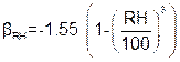
Submerged structures:
bHR = 0.25
|
RH |
Relative humidity |
|
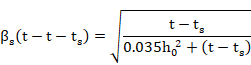
bs(t-ts) |
Coefficient for shrinkage development with time |
18-A.4.3 CEB-90 Code
18-A.4.3.1 Creep
In this code the creep coefficient is calculated as:

Where, j0 is the notional creep coefficient and bc coefficient to describe the development of creep with time after loading, t is the age of concrete in days at the moment considered and t0 the age of concrete at loading in days:
Where:
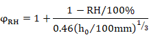
is a factor to allow for the effect of relative humidity on the notional creep coefficient.
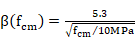
is a factor to allow for the effect of concrete strength on the notional creep coefficient.
is a factor to allow for the effect of concrete age at loading on the notional creep coefficient.
Where:
|
h0 |
Notional size in millimeters |
|
Ac |
Cross section area |
|
u |
Perimeter of the member in contact with the atmosphere |
|
fcm |
Mean compressive strength of concrete at the age of 28 days (MPa) |
The coefficient bc for the development of creep with time may be estimated from:
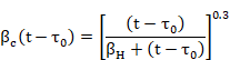
Where (t-t0 ) is the non-adjusted duration of loading in days and bH is a coefficient depending on the relative humidity (HR in %) and the notional member size h0 (mm):

18-A.4.3.2 Shrinkage
The shrinkage or swelling strains are calculated as:

where:
|
ecs0 |
Notional shrinkage coefficient |
|
bs |
Coefficient to describe the development of shrinkage with time |
|
t |
Age of concrete in days |
|
ts |
Age of concrete in days at the beginning of shrinkage |
The notional shrinkage coefficient may be obtained from:
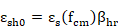
with


where bsc is a coefficient which depends on type of cement:
- 4 for slowly hardening cement (S)
- 5 for normal (N) or rapid hardening (R) cements
- 8 for rapid hardening high strength cements (RS).
The coefficient for the development of shrinkage with time may be estimated from:
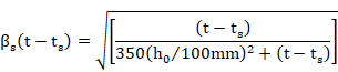
Where:
|
h0 |
Notional size in mm |
|
Ac |
Cross section area |
|
u |
Perimeter of the member in contact with the atmosphere |
|
(t-ts) |
Actual non-adjusted duration of shrinkage in days |

18-A.4.4 American Code ACI 209R-92
18-A.4.4.1 Creep
This code defines creep coefficient (the ratio of the creep strain to the initial
strain) through a monomial equation (Equation A-18) which includes the influence of different factors:
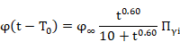
The average value suggested for j¥ is j¥ = 2.35
gI are correction factors for conditions other than the standard concrete conditions: loading age, volume-surface ratio method, ambient relative humidity, etc.
The correction factors to be applied are the following:
- Influence of loading age (t0 in days):
· For moist cured concrete:

· For steam cured concrete:

- Influence of ambient relative humidity (hr in %):

- Influence of volume-surface ratio (V/s in mm):

- Influence of slump (s in mm):

-
Influence of fine aggregate content ( is the ratio of the fine aggregate to total aggregate in kg/m3):
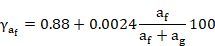
- Influence of air content (a in%):
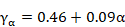
Creep strain takes into account Modulus of elasticity for each age.
18-A.4.4.2 Shrinkage
The equation for shrinkage deformation in ACI code is similar to the equation for creep:
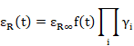

The average value suggested for eR¥ is eR¥ = 780 me
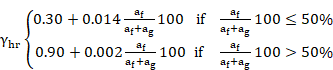
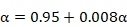
In the same way as for the creep model gI are correction factors for conditions other than the standard concrete conditions: volume-surface ratio method, ambient relative humidity, etc.
- Influence of ambient relative humidity (hr in %):

- Influence of volume-surface ratio (V/s in mm):

- Influence of slump (s in mm):

- Influence of fine aggregate content (af in kg/m3):
-
- Influence of cement content (c in kg/m3):

- Influence of air content (a in%):
18-A.4.5 Eurocode 2
18-A.4.5.1 Creep
In this code the creep coefficient is calculated as:

Where, j0 is notional creep coefficient and bc coefficient to describe the development of creep with time after loading, t is the age of concrete in days at the moment considered and t0 the age of concrete at loading in days:

where:
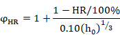
is a factor to allow for the effect of relative humidity on the notional creep coefficient.

is a factor to allow for the effect of concrete strength on the notional creep coefficient.
is a factor to allow for the effect of concrete age at loading on the notional creep coefficient.

is the notional size of member in millimeters where Ac is the cross section and u is the perimeter of the member in contact with the atmosphere.
The coefficient bc for the development of creep with time may be estimated from:
Where (t-t0) is the non-adjusted duration of loading in days and bH is a coefficient depending on the relative humidity (HR in %) and the notional member size h0 (mm):

18-A.4.5.2 Shrinkage
The shrinkage or swelling strains may be calculated from:
where:
|
ecs0 |
Notional shrinkage coefficient |
|
bs |
Coefficient to describe the development of shrinkage with time |
|
t |
Age of concrete in days |
|
ts |
Age of concrete in days at the beginning of shrinkage |
The notional shrinkage coefficient may be obtained from:
where


where bsc is a coefficient which depends on type of cement:
- 4 for slowly hardening cement (S)
- 5 for normal (N) or rapid hardening (R) cements
- 8 for rapid hardening high strength cements (RS).
The coefficient for the development of shrinkage with time may be estimated from:
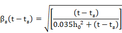
Where:
|
h0 |
Notional size in millimeters |
|
Ac |
Cross section area |
|
u |
Perimeter of the member in contact with the atmosphere |
|
(t-ts) |
Actual non-adjusted duration of shrinkage in days |
18-A.5 Non-Linear Beams
WARNING: This is a BETA feature. Difficulties may be encountered to achieve convergence in certain models and for some specific material laws (especially in those with a significantly different behavior in tension or in compression).
To use the BETA capabilities of CivilFEM it is necessary to activate them using the command KEYW,BETACIVI,1
18-A.5.1 Analysis procedure
The non linear beams calculation module carries out the substitution of each element real constants, in each calculation iteration, for the necessary values to create a fictitious section that with the linear stress-strain law of ANSYS, produces the same results that the real section with the real stress-strain law.
The analysis is conducted according to the following steps:
- Find strain values at nodes.
- Obtain real stresses (real law of the material) and linear stresses (linear stress-strain law with the elastic modulus contemplated by ANSYS).
- Calculate the reduction coefficients that will multiply the weights of the initial section to obtain the weights of the reduced section, and therefore the geometric properties of the reduced section (Static Equivalent Values).
- Obtain de geometric properties of the reduced section and substitute the real constants by the reduced values.
18-A.5.2 Strains and Curvatures
Strains at nodes are calculated from the end movements of the beam, taking into account the influence of temperature and the existence of offsets.
18-A.5.2.1 Strains due to Movements
Independently of the section’s internal composition and shape (homogeneous or composite), the computation of the strain e and curvature cy and cz values is achieved through the knowledge of the movements and rotations of the beam ends (obtained in ANSYS) using the following formulation:
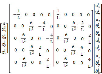
Or in abbreviated form:

In the above expression, only movements at the bar ends and the length of the beam are used exclusively. Movements have been referred to the local element axis.
This formula has been deduced for an element of constant section. For this reason, to take into account the geometrical differences between the two section ends, it is necessary to consider the obtained values in the following way:
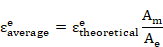
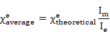
being:
e: end I or J of the beam.
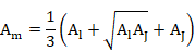

Starting from the above expression strains are calculated for the different section fibers. The strain value of the section’s fiber of local coordinates (y, z) is obtained by means of the following expression:

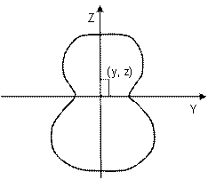 |
18-A.5.2.2 “Offset” influence
Movements and rotations of the beam ends obtained by ANSYS are always relative to the end nodes of the element and therefore the existence of offsets is not (displacements of the neutral axis with respect to the end nodes). Nevertheless, for the strains computation, it is required to know the movements and rotations of the center of gravity of the section.
Therefore, in the event that the considered bar element presents "offsets", defined by the arrays

Calling
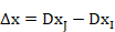
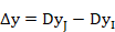
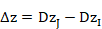
and with the notation of the accompanying figure, in which auxiliary axis have been adopted at node I, accumulating all the offset at node J we will obtain the following equations:
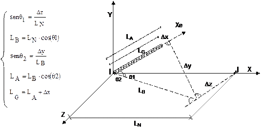 |
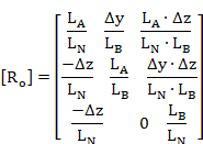
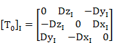
Being {u}P and {r}P the vectors with the movements at each node (obtained by ANSYS) and {ue}P and {re}P the vectors with the movements at the bar ends (P can be end I or J), both family of vectors are related by means of the following expression
{ue}P = [Ro] {u}P + [To]P [Ro] {r}P
{re}P = [Ro] {r}P
in which {r}I = {r}J , and therefore {re}I ={re}J are the movements and rotations used by the program to take into account the existence of “offsets” in the calculation of the strains described in the previous section. Substituting {ue}P and {re}P in the expression {e} = B.{u} the total strain can be obtained (considering the existence of offsets).
Matrices [Ro], [To]I and [To]J have the following expressions:
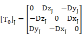
18-A.5.2.3 Temperature distribution effect in the section
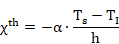
1. Two-dimensional Case
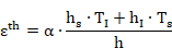
Considering Ts and TI as the temperatures in the section’s extreme fibers.
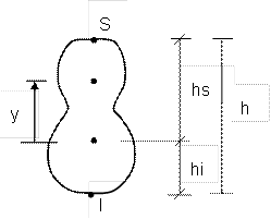 |
The strain of a fiber located at a certain height with respect to the center of gravity, is calculated using the following formula:

Comparing it with the distribution expected form the Navier hypothesis:
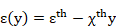
Therefore:
1. Three-dimensional Case
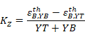
Starting from the temperature’s law of the section, strain values of the section can be obtained at different points of the section:
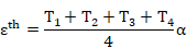
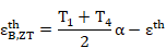
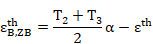
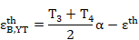
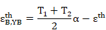
being:
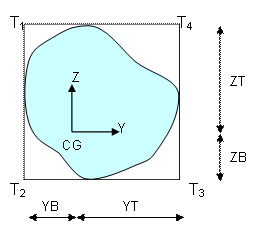 |
These values are the magnitudes labeled in ANSYS; EPTHDIR, EPTHBZT, EPTHBZB, EPTHBYT, EPTHBYB.
Where:
|
eth |
Thermal axial strain at one end. |
|
ethB,ZT |
Thermal strain at Z top fiber. |
|
ethB,ZB |
Thermal strain at Z bottom fiber. |
|
ethB,YT |
Thermal strain at Y top fiber. |
|
ethB,YB |
Thermal strain at Y bottom fiber. |
Starting from these strain values, total strains of the section can be obtained, using the following expressions:
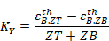

18-A.5.2.4 Strains
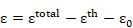
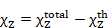
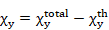
The procedure described in the previous sections to obtain the strains and curvatures from the nodal movement (taking the existence of “offsets” into account), provides the total strain and curvature values (etotal).
Nevertheless, in an isostatic structure, a temperature increment will produce movements and strains but not stresses. Of all strains suffered by the structure, only the fraction not coming from thermal effects may produce stresses and therefore strains coming from thermal (eth) actions will need to be discounted from strains coming from movements. Additionally, if the bar element is subjected to an initial strain, (eo) this strain is also discounted from the calculated total strain. Therefore, the formulation adopted by the program for the calculation of strains and curvatures is the following:
18-A.5.3 Calculation of Stresses in Fibers
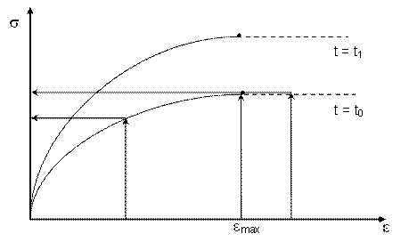
After the computation of strains, following the steps described above, real stresses can be obtained entering the actual stress-strain curve (e-s) of the material for the calculation period that is being conducted. That is, considering the adequate stress-strain curve for the material age in each step of the calculation period.
CivilFEM carries out an interpolation between the points defined in a curve as well as the available curves in order to obtain the stress that corresponds to any deformation value for any age. Nevertheless, if the value of the active time is less than the first age defined in the diagram, CivilFEM acts as if the material was not active and therefore its stress is zero for any deformation.
In the event that the obtained strain is greater than the maximum strain shown in the stress-strain diagram of the material, the stress is considered as constant after surpassing the point of maximum strain.
 |
Apart from the real stresses, linear stresses are also calculated based on the linear stress-strain law, in which the modulus of elasticity (E) contemplated by ANSYS is only considered for the calculation of the model.

The ratio of real stresses to linear stresses gives the Reduction Coefficient (n) for each point of the section.

18-A.5.4 Static Equivalent Values
18-A.5.4.1 Computation
Between iterations, the critical values of the section may change, modifying not only the area and moments of inertia but the position of the center of gravity and therefore the “offsets”.
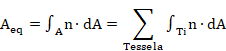
As previously stated, CivilFEM changes, at the end of each iteration, the values of the ANSYS real constants. To do so, the reduction coefficients (n) described in the earlier section are multiplied by the initial section weights to obtain the weights of the reduced section and therefore calculate the values of the geometric properties of the reduced section. The simplified formulas used are described hereafter:



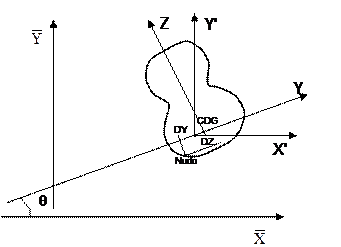 |
Where: Aeq= Area of the equivalent section (reduced)
Iyeq= Moment of inertia due to bending along the Y-axis of the equivalent section.
Izeq= Moment of inertia due to bending along the Z-axis of the equivalent section.
Iyzeq= Product of inertia of the equivalent section.
The moments of inertia are calculated relative to the inertia axes that pass through the center of gravity.
Additionally, the "offset" values are calculated with respect to the position of the node that defines the section (real constants DX, DY, DZ of ANSYS).
The center of gravity of the equivalent section is calculated using the classic formulation:
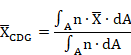
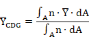
It is easily observed that the computation is based on comparing the situation of the section, in each iteration, with the situation of the initial section.
18-A.5.5 Specific Mass
If the area of the section changes, its mass and weight will automatically change in the same proportion. This will affect dynamic calculations and self-weight states as well as metric acceleration in static processes.
In order to correct this problem, the non-linear module modifies the ADDMASS real constant in those elements that include this option (BEAM44 and BEAM54). Two-hinged elements (LINK1, LINK8 and LINK10), which have been included in this module, do not allow this possibility. Therefore, they must be always inserted without mass and, if necessary, concentrating it at the nodes.
If the active time is less than the activation time of any of the defined materials, CivilFEM automatically performs the necessary adjustments so that the weight given to the section by the material is zero.
18-A.5.6 General Considerations
- Even though the cross sections must have a non-linear material defined, the model used for the analysis must be meshed using linear materials.
- Due to the fact that the non-linear module changes the values of the real constants in each equilibrium iteration, the use of the automatic control SOLCONTROL of ANSYS, could generate instabilities in the process.
- CivilFEM employs a system of elimination of instabilities by rounding up in the OFFSETS computation, not taking these offsets into account in the process while not exceeding a minimum value that is fixed proportionally to the corresponding dimension of the section. This value, which is taken by default as 10-9, can be controlled through the TOL configuration variable (see command ~CFCONFG).
- Occasionally, it can be beneficial to increment the maximum number of iterations (NEQIT). Recall that to do so, SOLCONTROL has to be previously deactivated.
- The appearance of offsets due to the use of different materials in the same section and the eventual formation of cracking phenomena in the process may cause convergence problems in elements with big depth/length ratio. Therefore, it is recommended to use elements with the following condition:
Finite element length ³ 0.20 ´ Depth of the section
- When an element suffers an increment or decrease of mass during the process, CivilFEM controls this phenomenon by means of the real constant ADDMASS (Beam 44 and BEAM54) but this constant applies to the total length of the beam and therefore it is necessary to take an average of the values obtained at each section end. This fact has to be taken into consideration so that the mesh used is sufficiently accurate.
- Given that elements used in non-linear calculations (LINK1, LINK8, LINK10, BEAM44, BEAM54) are created in ANSYS, their stiffness matrices have been used without changes. Thus, the solver equilibrium equations are formulated according to the stated stiffness matrices. The theoretical result of the forces at the ends of elements will be given by the integration of stresses in each point of the section. However, forces resulting from the non-linear calculation are the ones derived from the use of the stiffness matrices of the elements. Therefore forces may slightly vary in some cases.
18-A.5.7 Types of bar elements for non linear analysis
With respect to the non linear analysis of bar elements, these may present two different behaviors which can be define through the parameter KYNL (se command ~MEMBPRO)
This parameter can take the following values:
- KYNL = 0
The bar behaves as linear in the computation, but when analyzing the ENDS, such study is conducted considering the real non-linear behavior.
- KYNL = 1
The bar behavior is non linear, so much in the computation as in the study of its ENDS.
18-A.5.8 Types of non linear analysis
Two different possibilities exist when performing a non-linear analysis of bar elements in CivilFEM. These possibilities are controlled by the variable CFNLNTIP (see command ~CFCONFG).
- If CFNLNTIP = 0, the non-linear bars (NLSECCOM = 1) that correspond to the same group of real constants (sections) change simultaneously and consequently will always have the same static properties.
In this case, each time an iteration is carried out, the section properties change, equally affecting all bar elements susceptible of this change.
The criterion followed by CivilFEM is to leave the sections with the properties (real constants) obtained from the last modified element.
This line of work can save a lot of time but requires an adequate discretization of the model.
· If CFNLNTIP = 1, each non linear bar (NLSECCOM = 1) will have its own characteristic and therefore CivilFEM will have to generate automatically a new family of real constants for each beam. In this case, the computation is more precise although more costly in resources.
18-A.5.9 Moment curvature diagram
18-A.5.9.1 Non linear analysis with moment-curvature diagrams
Besides the calculation described in former sections, CivilFEM has the option of making a simplified non-linear calculation by using the moment-curvature diagrams of the sections used.
This type of calculation is limited to 2D structures and can be used with the same elements as in the general non-linear calculation (LINK1, LINK8, LINK20, BEAM44 and BEAM54).
As it will be shown in next sections, the calculation process is basically the same as in the general non-linear calculation, although the section is treated globally and not point by point.
In order to choose this type of calculation, it is necessary to change the MCKEY variable to MCKEY = 1 (by default MCKEY=0). See ~CFCONFG command.
18-A.5.9.2 Calculation of moment curvature diagrams
For a fixed value of an axil N, the moment curvature diagram is obtained by calculating the position of the neutral axis (fixed by the d variable) and the bending moment M for every curvature value c. These values obtained by equilibrium are points of the diagram. Assuming that concrete does not carry on tension:
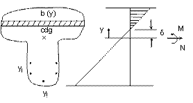 |
Since concrete does not sustain tension:
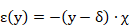
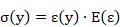


From the third equation, the value of d can be obtained as:
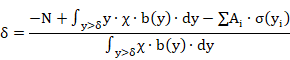
And back substituting into the second equation, the value of M can be calculated.
18-A.5.9.3 Pre-set diagrams
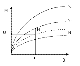
When a pre-set diagram of the section is defined, the calculations are carried out approximately, conforming the following steps:
- The starting point is defined by (c, e), curvature and axial strain.
- N is obtained from e and by interpolation in the curve, the value of M given for a certain c and N of the diagram.
- The INERTIA equivalent to the pair (c, M) is obtained.

- The real constants are modified and another iteration is carried out.
 |
18-A.5.9.4 Possibilities of diagram definition
Two options are available:
- Definition of the diagram by points.
- Definition of the real section diagram, calculated by CivilFEM. In this case the diagram is calculated on each iteration.