18-B.1               Introduction

From CivilFEM non linear and evolutive processes results described in Chapter 18 of this manual, the bridges and civil non Linearities module includes capabilities developed with the aim of facilitate and improve the analysis and design of bridges with ANSYS+CivilFEM.

The basic idea consists in generating, from the cross section and main axis definition in plan and elevation views, the structure target of study.

From this target, the module has been provided with the following utilities:

·         Utilities to generate common bridge cross sections

·         Utilities to generate de model in plan and elevation view. The mileage points which make up an imaginary line for the road central axis are defined. From the cross sections and layout definition, the program generates the complete model.

·         Automatic generation of the finite element model. It can be chosen between generating the solid finite element model or a shell element model or a beam element model.

·         Mobile loads generator. Once the load path is defined, loads are calculated automatically by the program, taking into account the vehicle type (rigid or flexible vehicle).

·         Overloads generator.

·         Utility for introducing the prestressed forces. The prestressed loads may be introduced as concentrated loads on the element’s nodes. The prestressed tension force is introduced at specific points along the tendon path and the program calculates an equivalent system of forces at each element’s node crossed by the tendon.

·         Capabilities to combine the load steps generated during the model analysis (traffic loads, overloads, prestressed forces, wind loads, etc).

To solve these problems, CivilFEM includes many capabilities in its bridge and civil non-Linearities module.

The way CivilFEM executes the analysis, and the supported element types are explained hereafter.

18-B.2               Element Types

CivilFEM the supported element types are the following:

Solid 3D	SOLID45, SOLID95, SURF154
Shell	SHELL43, SHELL63, SHELL181
Beam	BEAM44

The supported elements for the loads generation are the following:

3D Solid Model	SURF154
Shell Model	SURF154
Beam Model	BEAM3, BEAM4, BEAM44, BEAM54

 

 

18-B.3               Execution Process

CivilFEM bridge analysis performs the following steps:

• Geometry definition.
• Transverse cross section definition
• Bridge layout definition (elevation and plan view)
• Solid modeling and finite element model automatic generation.
• Loads generation: definition and/or family’s generation.
• Solution of individual load steps (prior to the combinations definition).
• Solution of load combinations.
• Structure reinforcement.

 

The model can also be generated independently without the bridge generation tools. In this case, the execution process would begin with the Loads generation.

 

18-B.4               Transverse cross sections

This module includes a library of typical bridge cross sections that contemplates the multiple geometric possibilities of the slab concrete cross sections (see ~BRSSLAB command) and of the box cross sections (see ~BRSBOX command).

18-B.4.1    Concrete slab cross sections

18-B.4.1.1       Types

·         Rectangular (RS)

It is the simplest section. It is defined by its dimensions B (width) and DEPTH (depth).

·         Trapezoidal (TS)

It is defined by its dimensions BBOT (lower width), BTOP (upper width), DEPTH (total depth) and TTOP (upper thickness).

·         Trapezoidal with overhang (TF)

It needs 6 parameters for its definition:

BBOT (lower width), BM (average width), BTOP (upper width), DEPTH (total depth), TBOT (lower thickness) and TTOP (upper thickness).

·         Symmetric polygonal with two corners (PS)

It needs 8 parameters for its definition, BBOT (lower width), BM1 and BM2 (intermediate width), BTOP (upper width), DEPTH (total depth), TBOT (lower thickness), TM (average thickness) and TTOP (upper thickness).

·         Asymmetric polygonal with two corners (PA)

It is the most general case. It requires two families of data, like the ones previously seen for a symmetric polygonal, which refer to the right and left hand side s of the section.

This section needs and arbitrary axis of reference for right and left measurements. At the intersection of this axis with the upper side the section coordinate system will be located. The axes need to be placed so that it intersects the upper and lower bases of the section, in order for all marked distances to be positive.

The different section’s topology and its corresponding geometric characteristics are represented in the following figure:

 

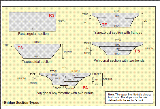
Figure 19.4-1 Concrete slab cross sections

18-B.4.1.2       Straight Outline

The lateral lines of the cross section contours are straight.

18-B.4.1.3       Hollow sections

Sections may be hollow. These circular holes will be defined by its center location and radius R. The transverse cross sections may vary along the structure but will need to have the same number of holes (see ~BRHL command for the holes definition).

18-B.4.1.4       Section axis

Each section has a coordinate system of axis Oxy associated to it. Its center is located at the center of the top base, being the Ox axis parallel to it when the section is symmetric, and at the point of intersection of the axis with the top side when the section is not symmetric.

 

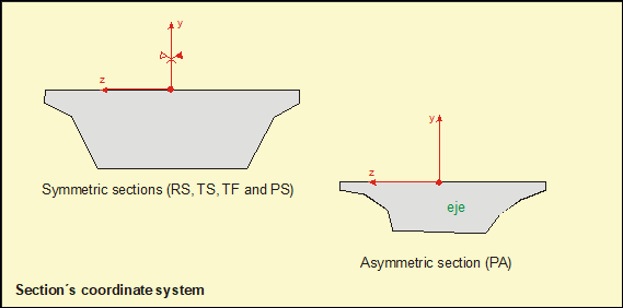
Figure 19.4-2 Section axis

18-B.4.2    Box cross sections

18-B.4.2.1       Types

Box bridge sections are made by an initial basic definition (see ~BRSBOX command) and by a succession of modifications about the geometry (see ~BRSMDF command).

This procedure allows a great variety of types and dimensions.

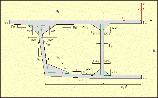
Figure 19.4-3 Box cross section

18-B.4.2.2       Section axis

Each section has a coordinate system of axis Oyz associated to it. Its center is located at the top base (without pumping) being the Oz axis parallel to it. If the section has an even number of cells, the system is located over the central web, and if the section has an odd number of cells, the system is located over the center of the central cell.

18-B.4.3    Angular units

CivilFEM bridge module allows 2 systems of angular measurements (sexagesimal degrees and radians). The definition of the angular units used is made through the ~BRANG command. The output data will be given in the chosen system.

 

18-B.5               Bridge layout definition

The procedure used for the bridge layout definition is the following:

-            Definition of the mileage points that represent the structure axis

-            Definition of plan and elevation layout

18-B.5.1    Definition of mileage points (MP’s)

Mileage points are points in the space supporting an imaginary line that constitutes the bridge axis, and will be used to define the structure by “placing” the cross sections over it. The mileage points definition is carried out using the ~BRINIP command.

18-B.5.2    Definition of bridge layout in plan view

To completely define in the space the structure’s axis, it is necessary to define the bridge stretches that connect these points in plan and elevation views.

In plan view, the mileage points line is a succession of user-defined stretches as straight segments, circular arcs or clothoid arcs.

18-B.5.2.1       Parametric equations of the clothoid

From the longitudinal arc radius (s) and the curvature radius (r), the following equations are used:

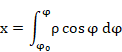
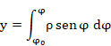
The relationship between s and r is established through the following equation

taking s₀ = 0 (clothoid center of symmetry), the following equation holds true

 

and therefore

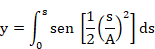
expressions which provide the clothoid parametric equations in the form of Fresnel integrals.

18-B.5.2.2       Plan view parameter definition

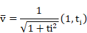
From the data introduced in ~BRADDPL command (used for plan view bridge definition) the characteristics of the stretch are obtained with the following formulation:

Case I: Straight stretch

The coordinates of the MP at the end of the stretch are:

 

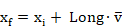
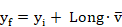
being

Case II: Circumference

The parameters are obtained from the bellow figure:

 

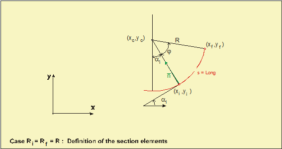
Figure 19.5-1 Circumference parameters

 

Case III: Clothoid

The parameters are obtained from the bellow figure:

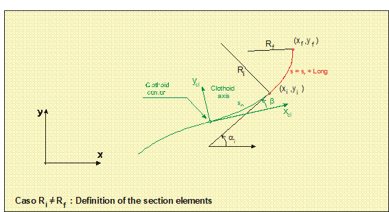
Figure 19.5-2 Clothoid parameters

18-B.5.3    Definition of bridge layout in elevation

The MP line in plan view may be defined as a sequence of straight or parabolic stretches. ~BRADDEL command must be used for the bridge layout definition in plan view.

For the analysis, the parabolic parameters coming from the stretches in elevation view are obtained from the figure shown bellow.

The parabola introduced has a vertical axis, with the annotation of the figure.

Where

 

 

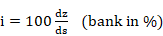
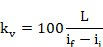
and L the longitudinal fillet (horizontal projection of the distance between points of MP extremes), the following relationships can be obtained:

 

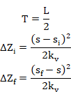
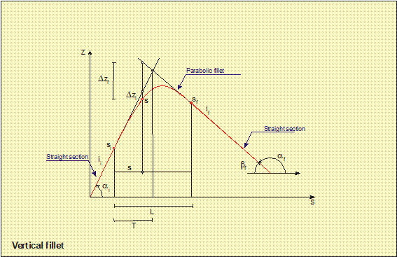
Figure 19.5-3 Bridge layout parameters in elevation view

18-B.5.4    Retrieving the bridge layout data

Data referred to the bridge layout most important properties for a particular mileage point may be retrieved with CivilFEM. Among these properties are coordinates of point, type of stretch in plan or elevation views, angle in plan or elevation views, curvature, etc. This information may be retrieved using ~BRIQR command.

18-B.5.5    Plot of surface road (line of mileage points)

Once the mileage points is defined, it can be plotted using ~BRSKTCH command.

This command creates a keypoint between every 2 lines generated, as well as a keypoint in the changing points of curve type, in plan and elevation views.

Lines and keypoints are saved into an assembly named BROUTE. This assembly can be later used to automatically generate the mobile loads and overloads (see sections 19.8-1 and 19.8-2). This assembly has the following components:

                                              BROUTEK - keypoints

                                                   BROUTEL - lines

 

 

18-B.6               Solid modeling and finite element model generation

This utility allows generating the complete geometrical model of the structure as well as the finite element model from the cross sections definition (its location, “offsets”, banks, etc) by using either solid elements, shell elements or beam elements.

18-B.6.1    Defining and assigning attributes

For the correct generation of the solid model and the finite element model of the structure, it is necessary to define a series of attributes. These attributes are described hereafter (see also the ~BRDEF command for attributes assignation):

18-B.6.1.1       Cross section number

Cross section number that will be assigned to the different mileage points (MP’s) forming the bridge. The cross sections may vary along the structure.

18-B.6.1.2        “Offsets”

Definition of the position of the intersection of the line of mileage points with the cross section plain (Y_offs, Z_offs), referred to the cross section coordinate system.

18-B.6.1.3        “Bank”

Possibility of defining the banks along the bridge. If the bank exists, the angle that the OZ cross section coordinate system axis forms with the horizontal line conforming the sketch represented in the bellow figure 19.6-1 can be defined.

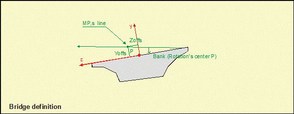
Figure 19.6-1 “Offsets” and “Banks” definition

18-B.6.1.4       Skew definition

This capability allows the definition of a skew angle of the cross section with respect to the road axis. The Ox axis of the cross-section coordinate system angle with respect to the bridge axis is defined (by default the cross section is taken perpendicular to the bridge axis). This angle pivots around the intersection of the mileage line and the cross section. The skew angle is not taken into account in the beam element model.

18-B.6.1.5       Hollow or solid sections

This capability allows to define hollow or solid sections from a particular mileage point. It allows to consider hollow sections as solid section at particular points of the structure (at supports, for example).

As previously commented, the transverse cross sections may vary along the bridge, with the restriction of having the same number of holes. Therefore, if solid and hollow cross sections are going to be used along the bridge layout, ~BRDEF command must be used.

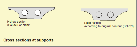
Figure 19.6-2 Hollow or solid cross sections

This option is not considered for box bridges.

18-B.6.2    Model generation

18-B.6.2.1       Interior divisions

After defining the attributes as described in the previous section, the bridge solid modeling and finite element generation is next.

With the aim of obtaining the passive reinforcement of slab concrete bridges, it is necessary to divide the cross section into compartments as indicated in figure 19.6-3:

This division is carried out automatically according to the following criteria:

1. A division will be located between two holes.
2. At least 2 divisions will be created between the last hole and the section’s edge.
3. In sections TF, PS and PA one division will be created at each point of banking change of the lateral sides of the section’s outline. These divisions cannot intersect any holes.
4. Stretch end section with largest division number, marks the number of divisions of the other section end.

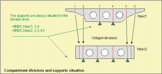
Figure 19.6-3 Divisions in slab cross sections

The division lines are identified by a number increment from left to right of the cross section. These lines can be moved using ~BRMVDL command. The program will check that the displaced line does not cut any holes and it is within the section outline.

18-B.6.2.2       Supports situation in slab concrete bridges

Supports will always be placed in the vertical divisions of the section (see figure 19.6-3). The location of these supports is entered with ~BRBC command indicating the cross section vertical line number associated to the support location. This command generates automatically one support in the keypoint belonging to the specified vertical line, restricting its movement with respect to the global Z axis (UZ=0) of the structure.

Additionally, If desired, supports can be defined or modified using the corresponding ANSYS commands (command DK).

This option is not considered for beam elements model.

18-B.6.2.3       Model generation

Model generation is carried out through the ~BRGEN command. This command offers five modeling options:

Option I- Only the solid model is created

In this case the model has been meshed using the corresponding ANSYS commands.

If this option is chosen, and later on the automatic generation of mobile loads and overloads of CivilFEM is going to be used, it would be necessary to create the components containing the deck nodes and elements that will be used in the loads generation.

Option II- Create the solid modeling and mesh only the first section

Option III- Create the solid modeling and the complete finite element model

When this option is chosen, the command generates the solid and finite element models. Moreover, assembly BDECK containing deck’s nodes is created and elements SURF154 are automatically generated when this option is chosen. This assembly can be later used in the automatic load and overload generation (see section 19.8).

Moreover, this command generates the following components:

 

NODES
CF_BR_DECK_NODE	Deck Nodes.
CF_BR_SECS_NODE_##	Cross section nodes in cross section local coordinate system (##).
ELEMENTS
CF_BR_DECK_SURF	Deck SURF154 elements.
CF_BR_SECS_ELEM_##	Cross section elements in cross section local coordinate system (##).
AREAS
CF_BR_DECK_AREA	Deck areas.
VOLUMES
CF_BR_SECS_VOLU_##	Volumes defined after the local coordinate system of the cross section (##).
CF_BR_HOLES_VOLU	Hole’s volumes.
ASSEMBLY
BDECK	Deck nodes and surface elements, for load application. It is formed by: CF_BR_DECK_NODE and CF_BR_DECK_SURF

                           ## Is the local axis system number created at each section.

 

Nodes and elements components are only created if the model is meshed.

Option IV- Create the solid modeling and the complete finite element model with shell elements

When this option is chosen, the command generates the solid and finite element models. Moreover, assembly BDECK containing deck’s nodes is created and elements SURF154 are automatically generated when this option is chosen. This assembly can be later used in the automatic load and overload generation (see section 19.8).

Moreover, this command generates the following components:

 

NODES
CF_BR_DECK_NODE	Deck Nodes.
CF_BR_SECS_NODE_##	Cross section nodes in cross section local coordinate system (##).
ELEMENTS
CF_BR_DECK_SURF	Deck SURF154 elements.
CF_BR_SECS_ELEM_##	Cross section elements in cross section local coordinate system (##).
AREAS
CF_BR_DECK_AREA	Deck areas.
CF_BR_SECS_AREA_##	Cross section areas in cross section local coordinate system (##).
ASSEMBLY
BDECK	Deck nodes and surface elements, for load application. It is formed by: CF_BR_DECK_NODE and CF_BR_DECK_SURF

                           ## Is the local axis system number created at each section.

 

This option is available only for box bridges.

Option V- Create the solid modeling and the finite element model with BEAM44 elements

The program creates a beam element model and automatically generates all cross sections and Beam&Shell properties needed.

 

ELEMENTS
CF_BR_ELEM	Beam elements.
NODES
CF_BR_NODE	Nodes of the model.
ASSEMBLY
BDECK	Deck nodes and elements, for load application. It is formed by: CF_BR_NODE and CF_BR_ELEM.

 

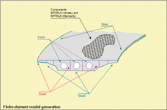
Figure 19.6-4 Model generation

18-B.7               Load definition structure

In the bridge analysis process, a great number of load steps are generated which later on have to be combined conforming the local codes. CivilFEM, through its combination module, allows to accomplishing this goal.

Nevertheless, due to the large number of load states handled in the combinations, this module establishes the concept of load families, which will be explained hereafter. This capability includes functionalities and commands that facilitate the user to work with load combinations.

Prior to the generation of start states, it is necessary to have the supports defined in such way that the load states created by CivilFEM, when generating the loads, can be included on them.

18-B.7.1    Families definition

Load families that can be later used in the combination module (as defined combinations) can be created.

A family is a group of load states, normally of the same topology. For example, the vehicles load would be a family formed by all loads created when the vehicles are placed in all the possible positions.

All the load steps belonging to a family are combined into one unique load step according to their nature (choosing adequately the combination parameters: favourable or unfavourable coefficients and number of start states to be added). The combined family can be later introduced as start state in other combinations.

It is necessary that the common nature of the start states belonging to a family allow to define the same favourable or unfavourable coefficients for all the family start states, otherwise each start state will constitute a different family.

The command that defines the family is ~BLFDF. This command defines the number assigned to the family, the favourable or unfavourable combination coefficients and the combination type that should be applied to the family generation. Depending on the chosen combination type, it may also be necessary to enter the number of start states to be considered (NADD). The possible combination types to be applied to the families are the same as the ones in the combination module (see chapter 6 of this manual for a detailed explanation of the different combination types):

 

(s) Program defined value

(u) User chosen value

The most general case is the latter (Selection with variable coefficients), the rest as particular cases of it.

As most frequent cases, we may mention the following ones:

 

One heavy vehicle in one line. Type INCOMPATIBLE or EXCLUSIVE.

Several heavy vehicles in one line SELECTION. NADD = Number of possible vehicles in one line.

Overload: The whole surface or part of the surface might be charged. Type COMPATIBLE. NADD = All expected loads.

Wind: Coefficients 1, -1 and NADD = all expected loads. Chooses only one start state among the possible ones. Type OPTION.

Seismic: Coefficients 1, -1 and NADD = all expected loads. Chooses only one start state among the possible ones. Type OPTION.

Prestressed loads: Coefficients 1, 1 and NADD = all expected loads. Type ADD.

 

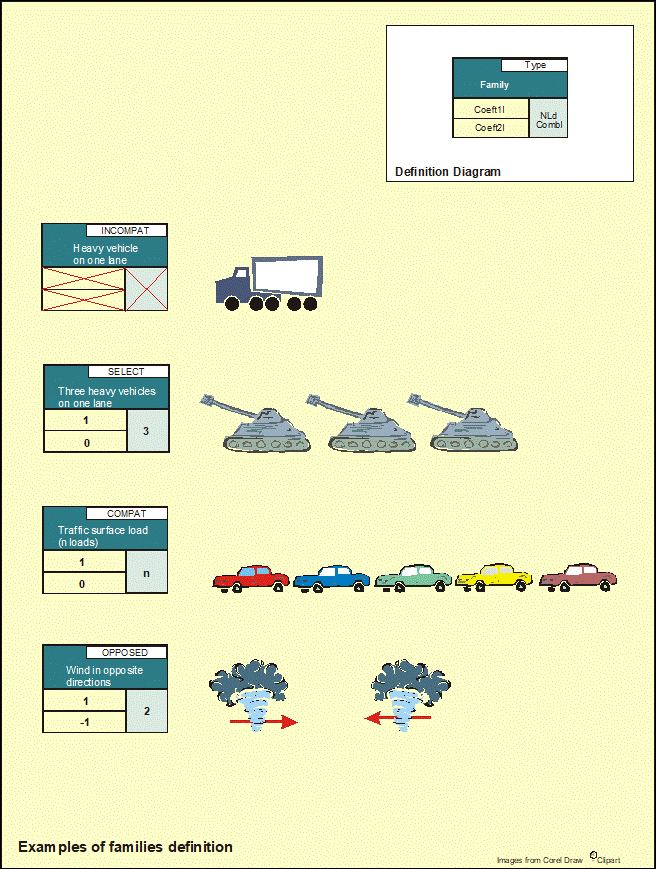
Figure 19.7-1 Families definition

18-B.7.2    Assigning user loads to families

CivilFEM defined loads (traffic loads, mobile or prestressed loads) are automatically assigned to families when the families are generated (it is an argument of the load generator command).

Nevertheless, the remaining user defined loads, such as wind, snow or seismic loads be assigned to previously defined families. Ones the load is defined using the corresponding ANSYS commands, the loads assignment is carried out through ~BLWRITE command indicating the family number to which the loads are assigned. This command executes the ~CFLSWRT command and introduces the created load in the indicated families. One same load can be assigned to 10 different families.

18-B.7.3    Solving a start state

Solving of simple start states is carried out through ~BLSOLVE command. This command performs the analysis all the start states contained in the families (mobile loads, overloads, prestressed and user loads).

 This command does not support restarts, nor birth and death of elements.

18-B.7.4    Conversion of families into combinations

Constructing the combinations from the families previously defined is carried out through ~BLF2CMB command. This command converts families in CivilFEM load combinations.

For example, family 1007 will be defined by commands:

~CMBDEF,1007,INCOMPAT   (which will represent the mobile load family)

~BLVR, 1007,... (that generates m start states)

~BLVR, 1007,... (that generates n start states)

~BLSOLVE (that will solve all m+n start states)

Then ~BLF2CMB command will automatically generate combination 1007 that will contain as “Start States” the m+n start states that belonged to the family of the same number, and that have been solve with ~BLSOLVE command. The combination will always have the same numbering as the family from which it has been generated.

Therefore, when ~BLF2CMB command is applied, all “start states” are automatically assigned to each generated combination, being only necessary the definition of the load combination targets.

Once this command is executed, it deletes the existing families and the corresponding commands of the CivilFEM load combination module (~TRGDEF command for target definition and ~COMBINE to perform the load combinations) must be used from this point.

Family’s main goal is to facilitate the generation of multiple loads that are going to be combined in order to obtain the structure’s worst case scenario.

On the other hand, if other loads have been defined independent from families, steps indicated in the CivilFEM load combination module must be followed (targets definition, start states definition, combination rule, etc).

18-B.8               Loads Generation

18-B.8.1    Traffic loads

18-B.8.1.1       Vehicle definition

The bridge load transfer is carried out by means of a rectangle of m x n points (see figure 19.8-1), which is defined with the following command structure:

~BLVST, Num

~BLVA, n, a₁, a₂, ..., a_n-1

~BLVB, m, b₁, b₂, ..., b_m-1

~BLVC, Type, d, start, end, xLoc, yLoc

~BLVD, j, Ini, P_Ini,j, P_Ini+1,j, ..., P_n,j

~BLVEND

Where

Num	-	Vehicle identification number. If this field is left blank, the program will assign a number immediately bigger than the last one.
n	-	Number of columns of different load scenarios.
m	-	Number of rows of different load scenarios.
Type	-	Vehicle type: 0 or blank – Rigid (Default value); 1 Flexible vehicle (vehicle which adapts to the path). Rigid or flexible vehicles may be defined (see figures 19.8-2 and 19.8-3). The path followed by the vehicle will have an effect in the analysis.
d	-	Free distance, prior to the vehicle crossing. This distance, defined as a rectangle of sides parallel to the ones defined by the vehicle, cannot be occupied by another vehicle. If this free zone is not defined, two vehicles will be able to touch each other (although they will not be able to occupy the same spot).
start	-	Part of the vehicle left outside the bridge at the beginning of the load generation.
end	-	Part of the vehicle left inside the bridge at the end of the load generation.
xLoc, yLoc	-	Coordinates of the vehicle’s center of reference, in order to place the vehicle in the path.
j	-	Row number in which the loads are defined (one for each column).
Ini	-	Column number in which the loads are defined.
Pij	-	Applied load at the point of intersection of column i with row j.

See commands aforementioned for a more detailed description of the way the vehicles may be defined. Once they are defined, vehicles can be deleted using command ~BLVDEL.

 

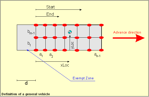
Figure 19.8-1 Vehicle definition

18-B.8.1.2       Mobile loads definition

Once the crossing vehicles are defined, traffic load generation is carried out automatically using command ~BLVR. Mobile loads, due to the fact that two or more vehicles cannot occupy more than one position at the same time, are considered as independent families. If it is only one vehicle, the combination type is incompatible, and in the case of several vehicles, the combination type is Selection with NADD equal to the number of vehicles that can be placed simultaneously. In this case, the mobile load generator creates a family containing the different possible positions of a vehicle along the path.

The mobile load generation needs the definition of the following parameters:

 

IdFam	-	Number to be assigned to the generated load family. The assigned family must be previously defined using ~BLFDF command. Otherwise, the program will display a warning message.
Id_FamH	-	Number assigned to the family of braking loads. If it is desired to consider the braking loads this family must have been defined previously. If this argument is left blank (or it is not introduced), this family is not created. This family will also not be created if values for parameters HL and HLMin described bellow are not introduced.
Id_Vehicle	-	Identification of the vehicle crossing along the bridge. The vehicle assigned number must be introduced using ~BLVST command.
CompLine	-	Component name. This component will contain a set of concatenated lines representing the road axis (line of mileage points). If ~BRSKTCH command has been used (which plots the defined path), the program will take as default value CompLine=BROUTEL.
AssemFE	-	Assembly name, containing the nodes and elements over which the loads will be applied. If the bridge finite element model has been created using ~BRGEN command, the program creates automatically this assembly and assigns AssemFE the following value AssemFE = BDECK (in case no other name has been defined). Otherwise, an assembly must be created using the corresponding ANSYS commands.
Dist	-	Displacement of the line component. It is measured with a positive sign towards de right, from the line advancing (or mileage points increment). The displacement is carried out normal to the lines components.
HL	-	Fraction of the weight transformed into a horizontal load (braking or starting load). It must be ³ 0 or blank. In this case it will be taken as zero.
HLMin	-	Minimum values of the aforementioned loads (for the whole vehicle. It must be ³ 0 or blank. In this case it will be taken as zero.

The family to which the vehicle’s loads are assigned will need to have the following characteristics:

a)    Only one vehicle

Type = Incompatible or Exclusive

Coef1 = 1   Coef2 = 0

NADD = 1

b)    n vehicles simultaneously

Type = Selection

Coef1 = 1   Coef2 = 0

NADD = n

The figures represented bellow indicates the path for the later assignment of mobile loads in rigid and flexible vehicles.

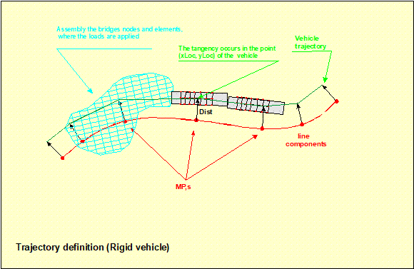
Figure 19.8-2 Path of rigid vehicles

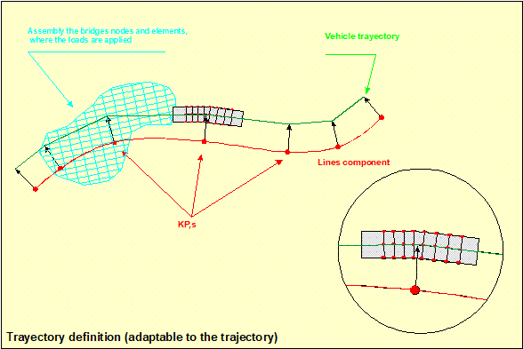
Figure 19.8-3 Path of flexible vehicles

A positive load over the wheel will be assigned to a load in the direction of the positive global Z-axis. The loads will be applied over all nodes of the structure affected by the vehicle path.

In case of performing a dynamic analysis with the vehicle loads, it’s necessary to activate this type of analysis (ANTYPE command) and define the following parameters with the ~BLVR command:

STTIME         Start time. For transient analysis. It will be ignored if velocity=0.

VELOCITY    Vehicle’s velocity. For transient analysis.

18-B.8.2    Surface loads generation

A surface load can be considered as a family of independent loads, although not excluded. This is why a COMPATIBLE behavior should be applied.

The generation of this type of families is carried out using the following commands (see figure 19.8-4):

~BLSST, Id_Fam, Id_FamH

~BLSA, m, d₁, d₂, ..., d_m

~BLSB, p, AssemKL, AssemFE, HL, HLMin

~BLSEND, UFZ

These commands generate rectangular loads of dimensions (s_i) x (d_j – d_j-1); where:

si	is the length of the stretch between keypoints that is automatically defined from the parameter AssemKL.
dj	is a measurement (with sign) along the direction normal to the bridge main axis. The positive sign is taken to the left, in the increasing direction of the mileage points (MP’s).
m	Number of dj parameters.
P	Surface load value.
Id_Fam	Family number to which the overloads will be assigned.
Id_FamH	Breaking loads family number. If this parameter is not defined, this family is not created.
AssemKL	Assembly name with keypoints and lines defining the road axis. If ~BRSKTCH command has been used (which plots the defined path), the program will take the following default value AssemKL=BROUTE.
AssemFE	Assembly name with nodes and elements over which the loads will be applied. If the bridge finite element model has been generated using ~BRGEN command, the program automatically creates this assembly and assigns AssemFE the following value AssemFE = BDECK (in case no other name has been defined). Otherwise, an assembly must be created using the corresponding ANSYS commands.
HL	Fraction of the weight transformed into a horizontal load (braking or starting load). It must be ³ 0 or blank. In this case it will be taken as zero.
HLMin	Minimum values of the aforementioned loads (for the whole vehicle It must be ³ 0 or blank. In this case it will be taken as zero.

 

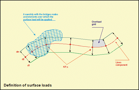
Figure 19.8-4 Overloads definition

A positive surface load will be assigned to a pressure in the normal direction towards inside of the structure. The loads will be applied over all elements of the structure.

The family to which the overloads are assigned will need to have the following characteristics:

Type = COMPAT

Coeft1 = Coeft2 = 1

NADD= all vehicles possible positions

Otherwise CivilFEM will display a warning message.

18-B.8.2.1       Beam elements model

The areas of the grid are projected on the beam elements, considering the dimensions of the cross sections. If the area is fully contained in the deck of the model, the complete load will be considered. If only part of the area overlaps with the beam model, equivalent loads will be placed on the beam to obtain the same reactions (forces and moments) as the ones the surface load on the overlapped area would create.

18-B.8.2.2       Solid elements model

For each of the areas of the loading grid, all the elements with their gravity center under the area will be loaded with the same load (pressure).

By default (UFZ = 0) the value of the surface load applied to all the elements is the one defined through the commands (constant value). This will have all the elements of the model loaded with the same surface load.

It is possible to apply a different load on the elements which will take into account the ratio between the area of the loaded elements and the area of the grid (UFZ = 1). This will obtain a total FZ reaction equal to the reaction produced by the surface load applied on the area of the grid. The elements under one loading area will have a constant surface pressure applied on them, different from the pressure applied on the elements of other area.

18-B.8.3    Prestressing cables loads

Loads due to active reinforcement, are introduced as concentrated loads, in the model’s nodes. This option is available only for solid element model.

18-B.8.3.1       Cable definition

Cable definition is carried out introducing the coordinates in the space of the points forming the cable, as well as the value of the tension force at these points. This capability is accessible through the following group of commands:

~BLCBST, IdCable

~BLCBPA, x, y, z, T, p1, p2, p3, q1, q2, q3

_…

~BLCBEND

Where:

IdCable	Cable identification number.
X, Y, Z	Point coordinates in the space.
T	Point stress (force units).
p1, p2, p3	Tangent vector to the point’s previous segment.
q1, q2, q3	Tangent vector to the point’s subsequent segment.

18-B.8.3.2       Cable path adjustment by means of cubic splines

CivilFEM will adjust cubic splines in stretches in without singular points.

Given a set of points in the space, {P₁, P₂, ..., P_N}, the objective is to obtain a set of cubic functions valid also between defined points, in such way that two adjacent curves not only go through the same point but so that they share the same tangent vector and curvature at that point location.

In order to solve this problem, it is necessary to know the tangent vectors at the set of end vectors. These vectors are represented by .

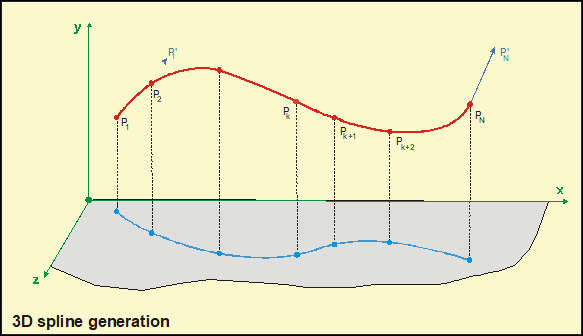
Figure 19.8-5 Generation of cubic splines

18-B.8.3.3       Introduction of the cables’ action over the structure

The procedure used by the program to introduce the forces transmitted by the cable to the structure is the following:

-          The cable is divided into separate parts in such way that each part lies inside an element and so that all parts will conform the cable.

-          The resultant of the cable action over the structure in this stretch is obtained. This resultant consists of two tangential forces at ends T1 and T2.

-          The equivalent forces system to set {T1, T2} referred to the element’s center of gravity is obtained.

This system is formed by three forces and three moments:

Its analysis is immediate, due to the following

being T_li the i component of the tension at end l (1 or 2), b_li the difference in elevation in the i direction between point l and the element center of gravity. .

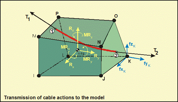
Figure 19.8-6 Transmission of cable actions

-          The objective is to find a system of forces, applied at the corner nodes of the elements that will equilibrate the system S_cdg.

Being n the element vertex number and G the center of gravity of an n mass unit system located at the vertices of the particular element, the system of forces {R, MR} equivalent to the prestressed force and reduced to the center of gravity is now represented (R is the resultant force and MR the moment with respect to G).

The objective is to look for a system of n forces {F_i} applied to the element nodes equilibrating the previous system.

Loads transference is done by using any of the following commands:

• ~BLPL assigns the cables to load families so they can be loaded alter (see ~BLSOLVE command). This command deletes all loads previously defined on the model.
• ~BLCBLD loads the model with the desired cables, but they are not assigned to a family and no previous loads are deleted.

18-B.8.4    Interaction with the combinations module

In the previous sections a set of commands that define the load steps and the subsequent load combination have been described.

These commands can be combined with the ones provided by the load combination module:

~CMBDEF	Defines a combination rule.
~COMBINE	Starts the calculation for all the combinations.
~STSTCFT	Defines the coefficients of a combination rule.
~STSTDEF	Defines the start states of a combination rule
~TRGDEF	Defines a Target.
~CMB	Reads the combined results corresponding to a specified target.

The user that is familiarized with CivilFEM combination module can use it to combine the bridge loads. To do so, it is only necessary to identify the loads that have been created inside each family (specially the ones generated by the commands: ~BLVR, moving loads; ~BLSST, overloads and ~BLCBST, cable actions). This data can be retrieved with the ~CFGET command.

The following commands can also be used:

~CMBINQ	Provides information about the coefficients and Start States used to obtain a Target at a point of the model.
~CMBLST	Lists the data of the combination rules.
~CMBSTAT	Lists the data of the combination module.
~TRGLST	Lists the Targets.

18-B.8.5    Loads in the beam element model

The same commands as for the solid or shell element model are applied. The commands do not change.

18-B.8.5.1       Overloads

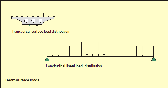
They are introduced as load per unit length through the beam directrix.

18-B.8.5.2       Moving loads

The moving loads are defined in the space, taking the Z coordinate as the vertical direction.

As for the solid element model, the moving loads generate two load families: one for the vertical component and other for the horizontal component. The vertical component is obtained by translating the load of each vehicle wheel to the closest point to the bridge directrix (beam), and introducing the corresponding torsional moment to the beam model.

The horizontal component is obtained as for the solid element model and it is translated to the beam model. The loads application is done by a load distribution among the nodes closest to the model.

The elements BEAM4, BEAM44, BEAM3 and BEAM54 can be applied. Although for the last two elements, as they are 2D elements, the applied loads can lead to actions over nonexistent degrees of freedom and, therefore, it would be ignored.

It’s very important to take into account the following aspects when introducing the loads:

• The vertical loads should be applied in the Z direction and the horizontal are tangent to the trajectory, specifying if the vehicle is rigid or flexible.
• The beam element model should have defined the Beam&Shell properties and the corresponding cross sections.
• The slab width corresponds to the cross section width according to the Z-axis of the section.
• The loads should be located over the beam width otherwise they are ignored.
• The variable beam cross-sections are contemplated supposing a linear variation.
• The model should be made of beam elements, one consecutive to the other and sharing the element ends. If more than two elements arrive in one node or the beam does not form a continuous structure, the applied loads can be different from the expected ones.
• All the elements of the component, over which the load will be applied, should be of the same type.

18-B.9               Construction process

18-B.9.1    Introduction

The bridges module has an option that allows to carry out the calculation of the multiple construction stages.

The construction method implemented in the present version of the program contemplates the construction process by phases. It means the construction of the bridge by placing the concrete and prestressing the cables segment by segment (more than one segment can be placed together).

18-B.9.2    Definition of the construction process

To carry out the construction process simulation, the type of construction process must be selected (see ~CPDEF command).

In addition, through the definition command, the number of steps that constitutes the construction process and all their possible actions should be defined. Each step will correspond to a load step in the solution time.

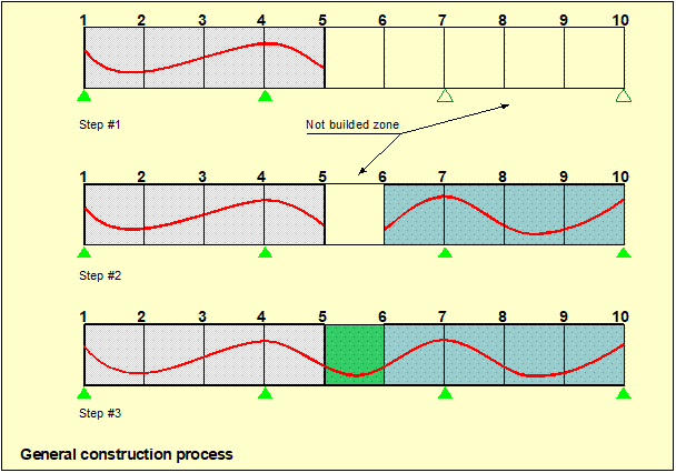
Figure 19.9.1 Construction process by phases

18-B.9.3    Data of each construction step

Each construction stage is associated to one step of the construction process. Therefore, all the properties and actions to be executed should be defined for each step (see ~CPSTDEF command).

Each construction step has a time associated to it in such way that it allows for the calculation of all the material ages that constitute the model. Besides that, for each step, the following must be defined:

-          Elements that should “die”

-          Elements that should “born”

-          Tendons that should be deactivated

-          Tendons

-          Actions

The birth and depth of elements and activation and deactivation of tendons are realized by the ~CPSTDEF command. This command creates some components in each step that contains the birth and depth elements.

A load step, with the same number as for the corresponding construction process step, should be created (see ~CFLSWRT command) in order to define the actions that will apply over the structure (gravity, forces, pressures, boundary conditions and so on).

18-B.9.4    Solution

The model is solved by the ~CFLSSLV command once the construction process as well as the properties in each step and the load steps with the corresponding loads are defined. This command works in a similar way of ANSYS' LSSOLVE command. It solves each one of the construction process steps and carries out all the operations of birth and depth of elements and activation and deactivation of tendons as well as updates the properties of the model to the actual calculation time.